The task of this section is data reconstruction, which is still the understanding of data

1. Data consolidation

In python, there are three functions that can merge data, namely concat, join, merge and join. Next, we will introduce the usage of these three functions.
1,pd.concat
pd.concat(objs, axis=0, join='outer', join_axes=None, ignore_index=False,
keys=None, levels=None, names=None, verify_integrity=False)
Description of common parameters:
objs: the data set to be merged, which can be a list composed of series or dataframe.
axis=0: merge by row by default. When axis=1, merge by column.
Join = 'outer': the default is external connection (Union of data). When join = 'inner', it is internal connection (intersection of data).
join_axes=None: this parameter is used to specify which axis to align the data according to.
ignore_index: when the parameter is True, the two tables will be aligned according to the column fields, and finally re assigned an index.

2,join
dataframe.join(other, on=None, how='left', lsuffix='', rsuffix='', sort=False)
Description of common parameters:
other: list form composed of dataframe, series or dataframe.
on=None: used to specify which column to merge based on. By default, it is merged based on index.
How = "left": the method of data merging. The default data is left connection. Other options of how are "right", "outer" and "inner".
lsuffix = '': string. Rename the duplicate column of the left data frame to "original column name + this string".
rsuffix = '': string. Rename the duplicate column of the data frame on the right to "original column name + this string".
sort=False: sort defaults to False. When it is True, the connection keys are arranged in order.

3,pd.merge
pd.merge(left, right, how='inner', on=None, left_on=None, right_on=None,left_index=False,
right_index=False,sort=False,suffixes=('_x', '_y'), copy=True,
indicator=False,validate=None)
Description of common parameters:
left: a dataframe.
right: the object to be merged is also a dataframe.
how = 'inner': the method of data consolidation. The default is inner. Other options are: 'left', 'right', 'outer'.
on=None: the column or index to be connected must exist in two dataframe s at the same time. If it is not specified, it defaults to the intersection of column names.
left_on=None，right_on=None: columns used as connection keys in datafarm on the left and right.
left_index=False, right_index=False: use the left and right row index references as their connection keys.

Summary of the characteristics of the three
concat: it can be used for vertical or horizontal splicing. The default is vertical splicing (i.e. line splicing). The connection mode is only internal connection and external connection.
merge: it can be used for vertical or horizontal splicing. The default is horizontal splicing. how = 'outer' can realize vertical splicing. The connection modes include inner, outer, left and right connections.
join: it can only be used for horizontal splicing. The connection methods include inner, outer, left and right connections. You can continue to use append to realize vertical splicing.

Take Titanic data as an example to show the usage of these three functions:

import numpy as np
import pandas as pd
from IPython.core.interactiveshell import InteractiveShell
InteractiveShell.ast_node_interactivity = "all"
#Loading of data
train_left_up=pd.read_csv("./data/train-left-up.csv")
train_left_up.head()
train_left_down=pd.read_csv("./data/train-left-down.csv")
train_left_down.head()
train_right_down=pd.read_csv("./data/train-right-down.csv")
train_right_down.head()
train_right_up=pd.read_csv("./data/train-right-up.csv")
train_right_up.head()

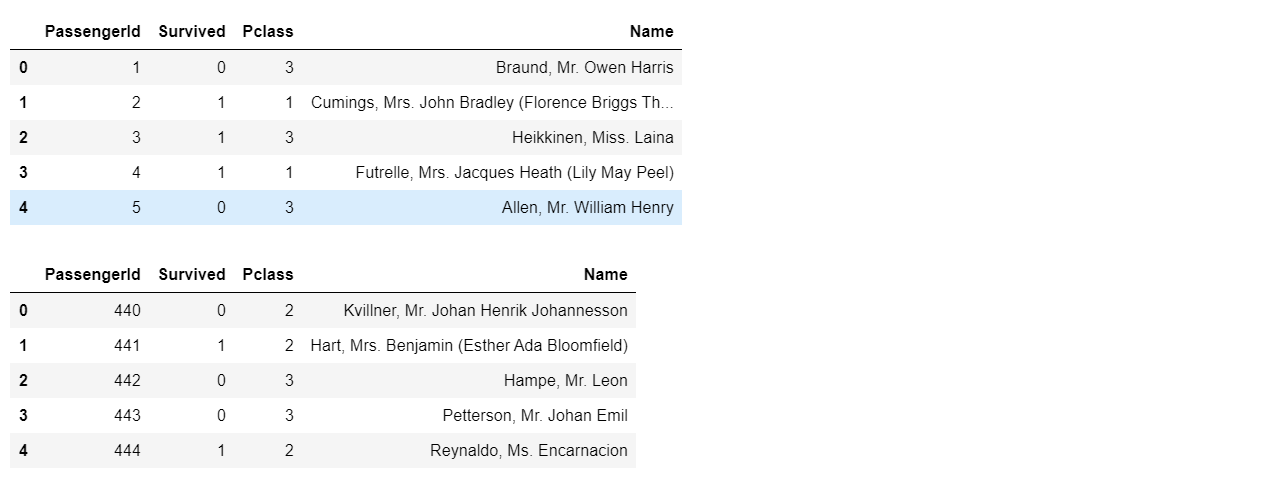
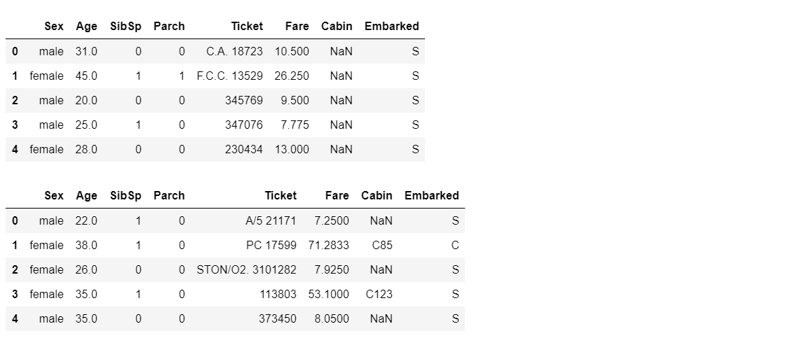
It is obvious that the four data sets divide the training set into four parts: upper left, lower left, upper right and lower right.

#Merge datasets using concat method
result_up=pd.concat([train_left_up,train_right_up],axis=1)
result_down=pd.concat([train_left_down,train_right_down],axis=1)
result=pd.concat([result_up,result_down])

#Use join and append methods to merge data sets
result_up=train_left_up.join(train_right_up)
result_down=train_left_down.join(train_right_down)
result=result_up.append(result_down)

#Use the methods of merge and append to merge data sets
result_up=pd.merge(train_left_up,train_right_up,left_index=True,right_index=True)
result_down=pd.merge(train_left_down,train_right_down,left_index=True,right_index=True)
result=result_up.append(result_down)

#Merge datasets using merge only
result_up=pd.merge(train_left_up,train_right_up,left_index=True,right_index=True)
result_down=pd.merge(train_left_down,train_right_down,left_index=True,right_index=True)
result=pd.merge(result_up,result_down,how='outer')

result

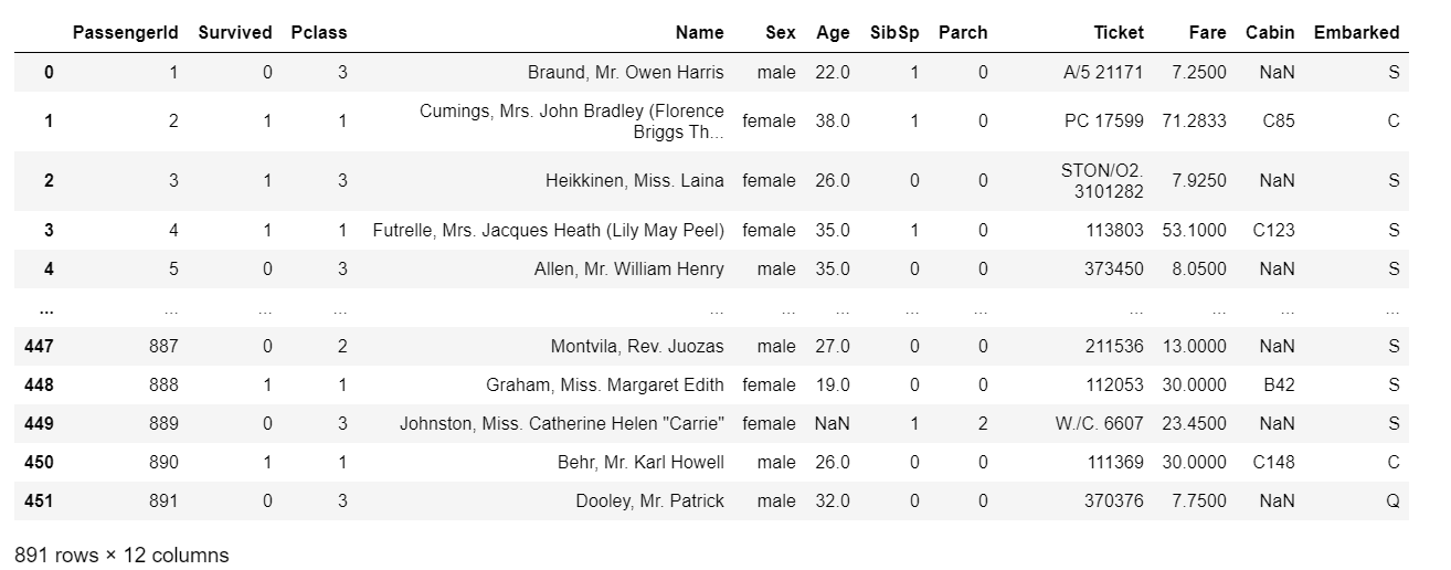
The final merged dataset is an 891 row, 12 column dataset, which is the same size as the training set we saw before.

2 change data to Series type data

The stack function can be used to convert the dataframe into series, which is convenient for us to process high-dimensional data in low-dimensional form.

result.stack().head(25)

You can see that the result is the beautified format of Series with MultilIndex index index.

3 data aggregation and operation

This section uses the groupby function to aggregate and calculate data.
Brief introduction to groupby function:
Group by can group data and apply functions to the grouped data for operation.
·groupby can be implemented in two ways:
1,df.groupby('key2')['key1']
2,df['key1'].groupby(df['key2'])
The above code indicates that the key1 column in df is grouped according to key2.
·groupby can directly calculate the grouped functions (taking the mean value as an example):
1,df.groupby('key2')['key1'].mean()
2,df['key1'].groupby(df['key2']).mean()

Next, we show the usage of groupby with several examples.

#1. Calculate the average ticket price for men and women on the Titanic
sex_fare=result['Fare'].groupby(result['Sex']).mean()
sex_fare

result:
Sex
female 44.479818
male 25.523893
Name: Fare, dtype: float64

#2. Count the survival of men and women on the Titanic
sex_survived=result['Survived'].groupby(result['Sex']).sum()
sex_survived

result:
Sex
female 233
male 109
Name: Survived, dtype: int64

#3. Calculate the number of survivors at different levels of the cabin
Pclass_survived=result['Survived'].groupby(result['Pclass']).sum()
Pclass_survived

result:
Pclass
1 136
2 87
3 119
Name: Survived, dtype: int64

Among them, tasks 1 and 2 can also be implemented simultaneously using the agg function

result.groupby('Sex').agg({'Fare':'mean','Survived':'sum'}).rename(columns=
                            {'Fare': 'fare_mean', 'Survived': 'survived_count'})

result:

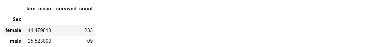
From the above results, we can get: the average ship price of women is 44.48, and the number of surviving women is 233; The average ship price for men is 25.52, and the number of surviving men is 109.

#4. Count the average cost of tickets of different ages in different levels of tickets
result['Fare'].groupby([result['Pclass'],result['Age']]).mean().head()

result:
Pclass Age
1 0.92 151.5500
2.00 151.5500
4.00 81.8583
11.00 120.0000
14.00 120.0000
Name: Fare, dtype: float64

#5,
#Get the total number of survivors at different ages, then find out the age of the highest number of survivors, and finally calculate the survival rate of the highest number of survivors
age_survived=result['Survived'].groupby(result['Age']).sum()
age_survived[age_survived.values==age_survived.max()]

people_survived=result['Survived'].sum()
survived_max=age_survived.max()/people_survived
survived_max
#

result:
Age
24.0 15
Name: Survived, dtype: int64

0.043859649122807015

The highest number of survivors was 24 years old, and a total of 15 survived. The survival rate at this age was 4.39%.