Differences between Logical Regression and Linear Regression
Linear regression can be applied to a similar number of training samples in different categories.If the number of training samples varies slightly from one category to another, it usually has little effect, but if the difference is large, the learning process will be confused.
Category imbalance refers to the situation where the number of training samples of different categories in the classification task varies greatly.
For example: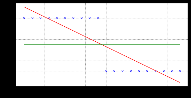
The graph shows whether toys are purchased and the relationship between age. Linear regression can be used to fit a straight line, labeling the purchased toys as 1, not as 0, and then taking a 0.5 value as a threshold to classify the categories.
You can see that on the way, the age distinction is about 19 years old.But when the data points are unbalanced, the thresholds are easily affected, as shown in the following figure:
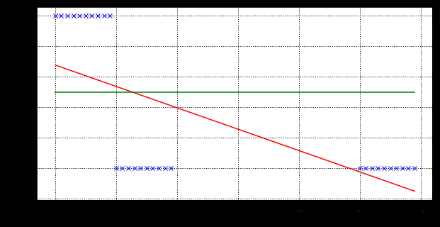
It can be seen that the true threshold of 0-value samples is still about 19 years old after the age shift to the higher age, but the threshold of the fitted curve is shifted backwards.Consider that the more negative samples there are, the more older people there are and the more severe the offset.But is that true?The fact is that neither 60 nor 80 years of age will buy toys. Adding a few 80 years of age will not affect the ability to see that after the age of the 0-value sample shifts to a higher age, the true threshold is still around 19 years of age, but the threshold of the fitted curve shifts backwards.Consider that the more negative samples there are, the more older people there are and the more severe the offset.But is that true?The fact is that neither 60 nor 80 years of age will buy toys. Increasing the number of 80 years of age will not affect the probability of people under 20 buying toys.However, since the original range of the fitted curve is () and the converted range is [0,1], the threshold is sensitive to variable offsets.The probability that people under 20 will buy toys.However, since the original range of the fitted curve is () and the converted range is [0,1], the threshold is sensitive to variable offsets.
Principles of Logical Regression
A common alternative is the logarithmic probability function, which is a "Sigmoid" function that converts a Z-value to a y-value close to 0 or 1, and its output value varies steeply around z=0.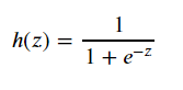
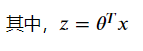
We can see that when z is greater than 0, the function is greater than 0.5; when the function is equal to 0, the function is equal to 0.5; and when the function is less than 0, the function is less than 0.5.If the probability of the target being classified into a certain class is expressed as a function, the following "unit step function" can be used to determine the type of data: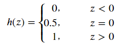
If Z is greater than 0, it is judged as normal; if less than 0, it is judged as negative; if equal to 0, it can be judged arbitrarily.Because the Sigmoid function is monotonic and differentiable, the Z-shaped range between functions (0, 1) can be used to simulate binary classification very well.
Regularization and Model Evaluation Indicators
Regularization
The over-fitting problem can be suppressed by adding a regularization function, the penalty term of theta, after the loss function.
L1 Regular:
J(θ)=1m∑i=1my(i)hθ(x(i))+(1−y(i))(1−hθ(x(i)))+λm∑i=1m∣θi∣
J(\theta) =\frac{1}{m}\sum^{m}_{i=1} y^{(i)}h_\theta (x^{(i)}) + (1-y^{(i)})(1-h_\theta (x^{(i)})) + \frac{\lambda}{m
}\sum^m_{i=1}|\theta_i|
J(θ)=m1i=1∑my(i)hθ(x(i))+(1−y(i))(1−hθ(x(i)))+mλi=1∑m∣θi∣
Δθil(θ)=1m∑i=1m(y(i)−hθ(x(i)))x(i)+λmsgn(θi)
\Delta_{\theta_i} l(\theta) = \frac{1}{m}\sum^m_{i=1}(y^{(i)} - h_\theta (x^{(i)}))x^{(i)} + \frac{\lambda}{m}sgn(\theta_i)
Δθil(θ)=m1i=1∑m(y(i)−hθ(x(i)))x(i)+mλsgn(θi)
The iteration function of the gradient descent method becomes,
θ:=θ−K′(θ)−λmsgn(θ)\theta:=\theta-K'(\theta)-\frac{\lambda}{m}sgn(\theta)θ:=θ−K′(θ)−mλsgn(θ)
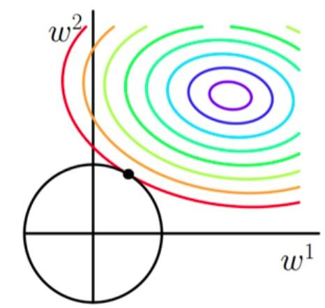
K( theta) is the original loss function. Since the symbol of the last term is determined by, you can see that the updated becomes smaller when is greater whenAs a result, the result of the L1 regularization adjustment will be more sparse (with more 0 values in the result vector).(See illustration, equivalent to finding the point on the contour that minimizes the diamond.)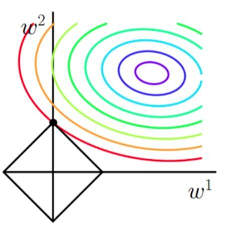
L2 Regular
J(θ)=1m∑i=1my(i)hθ(x(i))+(1−y(i))(1−hθ(x(i)))+λ2m∑i=1mθi2
J(\theta) =\frac{1}{m}\sum^{m}_{i=1} y^{(i)}h_\theta (x^{(i)}) + (1-y^{(i)})(1-h_\theta (x^{(i)})) + \frac{\lambda}{2m}\sum^m_{i=1}\theta_i^2
J(θ)=m1i=1∑my(i)hθ(x(i))+(1−y(i))(1−hθ(x(i)))+2mλi=1∑mθi2
Δθil(θ)=1m∑i=1m(y(i)−hθ(x(i)))x(i)+λmθi
\Delta_{\theta_i} l(\theta) = \frac{1}{m}\sum^m_{i=1}(y^{(i)} - h_\theta (x^{(i)}))x^{(i)} + \frac{\lambda}{m}\theta_i
Δθil(θ)=m1i=1∑m(y(i)−hθ(x(i)))x(i)+mλθi
The iteration function of the gradient descent method becomes,
θ:=θ−K′(θ)−2λmθ\theta:=\theta-K'(\theta)-\frac{2\lambda}{m}\thetaθ:=θ−K′(θ)−m2λθ
() is the original loss function, the most important one determines the penalty on the parameters. The greater the penalty, the smaller and dispersed parameters of the final result vector generally, avoiding the individual parameters having a greater impact on the whole function.(See illustration, equivalent to finding the point on the contour that minimizes the circle)
python implementation
use skearn
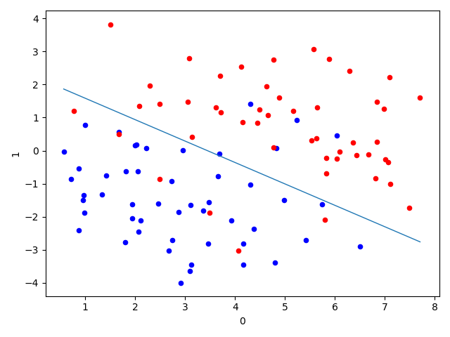
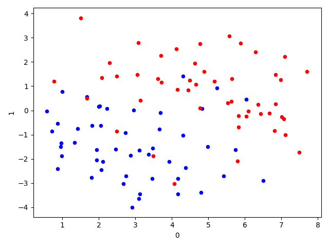
import pandas as pd
import matplotlib.pyplot as plt

df_X = pd.read_csv('./logistic_x.txt', sep='\ +', header=None, engine='python')  # Read X Value
ys = pd.read_csv('./logistic_y.txt', sep='\ +', header=None, engine='python')  # Read y Value
ys = ys.astype(int)  # Convert ys ys to an integer data type
df_X['label'] = ys[0].values  # Label X as y-values
ax = plt.axes()
# Draw the X-point location in a two-dimensional graph to visually see the distribution of data points
df_X.query('label == 0').plot.scatter(x=0, y=1, ax=ax, color='blue')
df_X.query('label == 1').plot.scatter(x=0, y=1, ax=ax, color='red')
plt.show()
from __future__ import print_function
import pandas as pd
import matplotlib.pyplot as plt
import numpy as np
from sklearn.linear_model import LogisticRegression

df_X = pd.read_csv('./logistic_x.txt', sep='\ +',header=None, engine='python')  # Read X Value
ys = pd.read_csv('./logistic_y.txt', sep='\ +',header=None, engine='python')  # Read y Value
ys = ys.astype(int)
df_X['label'] = ys[0].values  # Label X as y-values
# Extracting data for learning
Xs = df_X[[0, 1]].values
Xs = np.hstack([np.ones((Xs.shape[0], 1)), Xs])
"""
[Stitching Array Method)
np.hstack-Stack arrays in sequence horizontally (column wise).
np.vstack-Stack arrays in sequence vertically (row wise).
https://docs.scipy.org/doc/numpy/reference/generated/numpy.hstack.html
"""
ys = df_X['label'].values

lr = LogisticRegression(fit_intercept=False)  # Because the value of the intercept item has been previously merged into the variable, there is no need for the intercept item to be set here
lr.fit(Xs, ys)  # fitting
score = lr.score(Xs, ys)  # Result Evaluation
print("Coefficient: %s" % lr.coef_)
print("Score: %s" % score)

ax = plt.axes()
df_X.query('label == 0').plot.scatter(x=0, y=1, ax=ax, color='blue')
df_X.query('label == 1').plot.scatter(x=0, y=1, ax=ax, color='red')

_xs = np.array([np.min(Xs[:,]), np.max(Xs[:, 1])])
# The data is plotted in two-dimensional graphics, and the data area is divided using the parameter results learned as the threshold value.
_ys = (lr.coef_[0][0] + lr.coef_[0][1] * _xs) / (- lr.coef_[0][2])
plt.plot(_xs, _ys, lw=1)
logistic regression
import pandas as pd
import matplotlib.pyplot as plt
import numpy as np

df_X = pd.read_csv('./logistic_x.txt', sep='\ +', header=None, engine='python')  # Read X Value
ys = pd.read_csv('./logistic_y.txt', sep='\ +', header=None, engine='python')  # Read y Value
ys = ys.astype(int)  # Convert ys ys to an integer data type
df_X['label'] = ys[0].values  # Label X as y-values
# Extracting data for learning
Xs = df_X[[0, 1]].values
Xs = np.hstack([np.ones((Xs.shape[0], 1)), Xs])
"""
[Stitching Array Method)
np.hstack-Stack arrays in sequence horizontally (column wise).
np.vstack-Stack arrays in sequence vertically (row wise).
https://docs.scipy.org/doc/numpy/reference/generated/numpy.hstack.html
"""
ys = df_X['label'].values

class LGR_GD():
    def __init__(self):
        self.w = None
        self.n_iters = None

    def fit(self, X, y, alpha=0.03, loss=1e-10):  # Set the step size to 0.02 and the criterion for determining convergence is 1 E-10
        y = y.reshape(-1, 1)  # Reshape the dimensions of y values for matrix operations
        [m, d] = np.shape(X)  # Dimension of independent variable
        self.w = np.zeros((1, d))  # Set the initial value of the parameter to 0
        tol = 1e5
        self.n_iters = 0
        # ============================= show me your code =======================
        while tol > loss:  # Set Convergence Conditions
            # Calculating Sigmoid Function Results
            sigmoid = 1 / (1 + np.exp(-X.dot(self.w.T)))
            theta = self.w + alpha * np.mean(X * (y - sigmoid), axis=0)  # Iterate the value of the TA
            tol = np.sum(np.abs(theta - self.w))  # Calculate loss value
            self.w = theta
            self.n_iters += 1  # Number of update iterations
        # ============================= show me your code =======================

    def predict(self, X):
        # Prediction of new independent variables with fitted parameter values
        y_pred = X.dot(self.w)
        return y_pred


if __name__ == "__main__":
    lr_gd = LGR_GD()
    lr_gd.fit(Xs, ys)

    ax = plt.axes()

    df_X.query('label == 0').plot.scatter(x=0, y=1, ax=ax, color='blue')
    df_X.query('label == 1').plot.scatter(x=0, y=1, ax=ax, color='red')

    _xs = np.array([np.min(Xs[:, 1]), np.max(Xs[:, 1])])
    _ys = (lr_gd.w[0][0] + lr_gd.w[0][1] * _xs) / (- lr_gd.w[0][2])
    plt.plot(_xs, _ys, lw=1)
    plt.show()