
Feather low is a 3D scan based image that I want to share with you today. The article will divide and explain the whole code. After reading it completely, I believe you will gain something.
Welcome to "Yufeng codeword"
catalogue
3.3 establishment of training and validation data sets
4.1 definition of 3D convolutional neural network
5. Use the model for prediction
1. Project introduction
This example will show the steps required to build a 3D convolutional neural network (CNN) to predict the presence of viral pneumonia in computed tomography (CT) scans. 2D CNN is usually used to process RGB images (3 channels). 3D CNN is only a 3D equivalent: it takes 3D volume or 2D frame sequence (such as slices in CT scan) as input, so 3D CNN is a powerful model for learning the representation of volume data.
2. API preparation
import os
import zipfile
import numpy as np
import tensorflow as tf

from tensorflow import keras
from tensorflow.keras import layers
3. Data set preparation
3.1 downloading data
Download MosMedData: chest CT scan with COVID-19 related findings
In this example, we use MosMedData: Chest CT Scans with COVID-19 Related Findings . This data set contains lung CT scans with COVID-19 related findings and none.
We will use the relevant radiological findings of CT scans as markers to establish a classifier to predict the presence of viral pneumonia. Therefore, the task is a binary classification problem.
# Download url of normal CT scans.
url = "https://github.com/hasibzunair/3D-image-classification-tutorial/releases/download/v0.2/CT-0.zip"
filename = os.path.join(os.getcwd(), "CT-0.zip")
keras.utils.get_file(filename, url)

# Download url of abnormal CT scans.
url = "https://github.com/hasibzunair/3D-image-classification-tutorial/releases/download/v0.2/CT-23.zip"
filename = os.path.join(os.getcwd(), "CT-23.zip")
keras.utils.get_file(filename, url)

# Make a directory to store the data.
os.makedirs("MosMedData")

# Unzip data in the newly created directory.
with zipfile.ZipFile("CT-0.zip", "r") as z_fp:
    z_fp.extractall("./MosMedData/")

with zipfile.ZipFile("CT-23.zip", "r") as z_fp:
    z_fp.extractall("./MosMedData/")
3.2 data preprocessing
These files are provided in Nifti format with the extension nii. To read the scan results, we use the nibabel package. You can install packages via pip install nibabel. CT scans store the original voxel intensity in Hounsfield units (HU). In this dataset, they range from - 1024 to more than 2000. Bones above 400 have different radiation intensities, so they are used as a higher limit. Thresholds between - 1000 and 400 are typically used for normalized CT scans.
To process data, we do the following:
- We first rotate the volume 90 degrees, so the direction is fixed
- We scale the HU value between 0 and 1.
- We adjust the size of width, height and depth.
Here, we define several auxiliary functions to process data. These features will be used when building training and validation datasets.
import nibabel as nib

from scipy import ndimage


def read_nifti_file(filepath):
    """Read and load volume"""
    # Read file
    scan = nib.load(filepath)
    # Get raw data
    scan = scan.get_fdata()
    return scan


def normalize(volume):
    """Normalize the volume"""
    min = -1000
    max = 400
    volume[volume < min] = min
    volume[volume > max] = max
    volume = (volume - min) / (max - min)
    volume = volume.astype("float32")
    return volume


def resize_volume(img):
    """Resize across z-axis"""
    # Set the desired depth
    desired_depth = 64
    desired_width = 128
    desired_height = 128
    # Get current depth
    current_depth = img.shape[-1]
    current_width = img.shape[0]
    current_height = img.shape[1]
    # Compute depth factor
    depth = current_depth / desired_depth
    width = current_width / desired_width
    height = current_height / desired_height
    depth_factor = 1 / depth
    width_factor = 1 / width
    height_factor = 1 / height
    # Rotate
    img = ndimage.rotate(img, 90, reshape=False)
    # Resize across z-axis
    img = ndimage.zoom(img, (width_factor, height_factor, depth_factor), order=1)
    return img


def process_scan(path):
    """Read and resize volume"""
    # Read scan
    volume = read_nifti_file(path)
    # Normalize
    volume = normalize(volume)
    # Resize width, height and depth
    volume = resize_volume(volume)
    return volume
Let's read the path of CT scan from the class directory.
# Folder "CT-0" consist of CT scans having normal lung tissue,
# no CT-signs of viral pneumonia.
normal_scan_paths = [
    os.path.join(os.getcwd(), "MosMedData/CT-0", x)
    for x in os.listdir("MosMedData/CT-0")
]
# Folder "CT-23" consist of CT scans having several ground-glass opacifications,
# involvement of lung parenchyma.
abnormal_scan_paths = [
    os.path.join(os.getcwd(), "MosMedData/CT-23", x)
    for x in os.listdir("MosMedData/CT-23")
]

print("CT scans with normal lung tissue: " + str(len(normal_scan_paths)))
print("CT scans with abnormal lung tissue: " + str(len(abnormal_scan_paths)))
3.3 establishment of training and validation data sets
Read, scan and assign labels from the class directory. The scan is down sampled to have a shape of 128x128x64. Rescale the original HU value to a range of 0 to 1. Finally, the data set is divided into training and verification subsets.
# Read and process the scans.
# Each scan is resized across height, width, and depth and rescaled.
abnormal_scans = np.array([process_scan(path) for path in abnormal_scan_paths])
normal_scans = np.array([process_scan(path) for path in normal_scan_paths])

# For the CT scans having presence of viral pneumonia
# assign 1, for the normal ones assign 0.
abnormal_labels = np.array([1 for _ in range(len(abnormal_scans))])
normal_labels = np.array([0 for _ in range(len(normal_scans))])

# Split data in the ratio 70-30 for training and validation.
x_train = np.concatenate((abnormal_scans[:70], normal_scans[:70]), axis=0)
y_train = np.concatenate((abnormal_labels[:70], normal_labels[:70]), axis=0)
x_val = np.concatenate((abnormal_scans[70:], normal_scans[70:]), axis=0)
y_val = np.concatenate((abnormal_labels[70:], normal_labels[70:]), axis=0)
print(
    "Number of samples in train and validation are %d and %d."
    % (x_train.shape[0], x_val.shape[0])
)
3.4 data enhancement
During training, CT scanning can also be enhanced by rotating at any angle. Since the data is stored in the three-level tensor of the shape (sample, height, width, depth), we add a dimension of dimension 1 on axis 4 to enable 3D convolution of the data. Therefore, the new shape is (sample, height, width, depth, 1). There are also various preprocessing and expansion technologies. Please refer to relevant materials. This example shows some simple introduction and enhancement technologies.
import random

from scipy import ndimage


@tf.function
def rotate(volume):
    """Rotate the volume by a few degrees"""

    def scipy_rotate(volume):
        # define some rotation angles
        angles = [-20, -10, -5, 5, 10, 20]
        # pick angles at random
        angle = random.choice(angles)
        # rotate volume
        volume = ndimage.rotate(volume, angle, reshape=False)
        volume[volume < 0] = 0
        volume[volume > 1] = 1
        return volume

    augmented_volume = tf.numpy_function(scipy_rotate, [volume], tf.float32)
    return augmented_volume


def train_preprocessing(volume, label):
    """Process training data by rotating and adding a channel."""
    # Rotate volume
    volume = rotate(volume)
    volume = tf.expand_dims(volume, axis=3)
    return volume, label


def validation_preprocessing(volume, label):
    """Process validation data by only adding a channel."""
    volume = tf.expand_dims(volume, axis=3)
    return volume, label
When defining the training and validation data loader, the training data will be transferred through the and enhancement function, which will randomly rotate the volume at different angles. Notice that both the training and validation data have been rescaled to values between 0 and 1.
# Define data loaders.
train_loader = tf.data.Dataset.from_tensor_slices((x_train, y_train))
validation_loader = tf.data.Dataset.from_tensor_slices((x_val, y_val))

batch_size = 2
# Augment the on the fly during training.
train_dataset = (
    train_loader.shuffle(len(x_train))
    .map(train_preprocessing)
    .batch(batch_size)
    .prefetch(2)
)
# Only rescale.
validation_dataset = (
    validation_loader.shuffle(len(x_val))
    .map(validation_preprocessing)
    .batch(batch_size)
    .prefetch(2)
)
Visual CT enhanced image
import matplotlib.pyplot as plt

data = train_dataset.take(1)
images, labels = list(data)[0]
images = images.numpy()
image = images[0]
print("Dimension of the CT scan is:", image.shape)
plt.imshow(np.squeeze(image[:, :, 30]), cmap="gray")
Because there are many slices in CT scan, they are arranged and displayed in sequence
def plot_slices(num_rows, num_columns, width, height, data):
    """Plot a montage of 20 CT slices"""
    data = np.rot90(np.array(data))
    data = np.transpose(data)
    data = np.reshape(data, (num_rows, num_columns, width, height))
    rows_data, columns_data = data.shape[0], data.shape[1]
    heights = [slc[0].shape[0] for slc in data]
    widths = [slc.shape[1] for slc in data[0]]
    fig_width = 12.0
    fig_height = fig_width * sum(heights) / sum(widths)
    f, axarr = plt.subplots(
        rows_data,
        columns_data,
        figsize=(fig_width, fig_height),
        gridspec_kw={"height_ratios": heights},
    )
    for i in range(rows_data):
        for j in range(columns_data):
            axarr[i, j].imshow(data[i][j], cmap="gray")
            axarr[i, j].axis("off")
    plt.subplots_adjust(wspace=0, hspace=0, left=0, right=1, bottom=0, top=1)
    plt.show()


# Visualize montage of slices.
# 4 rows and 10 columns for 100 slices of the CT scan.
plot_slices(4, 10, 128, 128, image[:, :, :40])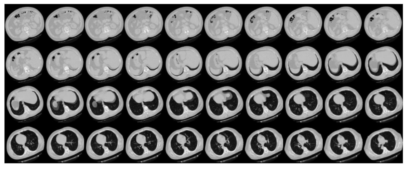
4 model construction
4.1 definition of 3D convolutional neural network
To make the model easier to understand, we construct it into blocks. The architecture of 3D CNN used in this example is based on this paper of
def get_model(width=128, height=128, depth=64):
    """Build a 3D convolutional neural network model."""

    inputs = keras.Input((width, height, depth, 1))

    x = layers.Conv3D(filters=64, kernel_size=3, activation="relu")(inputs)
    x = layers.MaxPool3D(pool_size=2)(x)
    x = layers.BatchNormalization()(x)

    x = layers.Conv3D(filters=64, kernel_size=3, activation="relu")(x)
    x = layers.MaxPool3D(pool_size=2)(x)
    x = layers.BatchNormalization()(x)

    x = layers.Conv3D(filters=128, kernel_size=3, activation="relu")(x)
    x = layers.MaxPool3D(pool_size=2)(x)
    x = layers.BatchNormalization()(x)

    x = layers.Conv3D(filters=256, kernel_size=3, activation="relu")(x)
    x = layers.MaxPool3D(pool_size=2)(x)
    x = layers.BatchNormalization()(x)

    x = layers.GlobalAveragePooling3D()(x)
    x = layers.Dense(units=512, activation="relu")(x)
    x = layers.Dropout(0.3)(x)

    outputs = layers.Dense(units=1, activation="sigmoid")(x)

    # Define the model.
    model = keras.Model(inputs, outputs, name="3dcnn")
    return model


# Build model.
model = get_model(width=128, height=128, depth=64)
model.summary()
4.2 training model
# Compile model.
initial_learning_rate = 0.0001
lr_schedule = keras.optimizers.schedules.ExponentialDecay(
initial_learning_rate, decay_steps=100000, decay_rate=0.96, staircase=True
)
model.compile(
loss="binary_crossentropy",
optimizer=keras.optimizers.Adam(learning_rate=lr_schedule),
metrics=["acc"],
)
# Define callbacks.
checkpoint_cb = keras.callbacks.ModelCheckpoint(
"3d_image_classification.h5", save_best_only=True
)
early_stopping_cb = keras.callbacks.EarlyStopping(monitor="val_acc", patience=15)
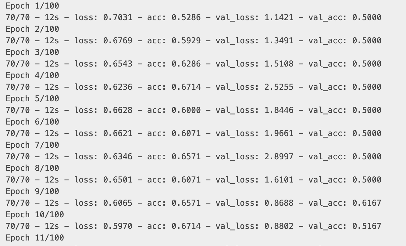
# Train the model, doing validation at the end of each epoch
epochs = 100
model.fit(
train_dataset,
validation_data=validation_dataset,
epochs=epochs,
shuffle=True,
verbose=2,
callbacks=[checkpoint_cb, early_stopping_cb],
)
4.3 validation model
The model accuracy and loss of training and verification sets are drawn here. Since the validation set is class balanced, accuracy provides a fair representation of model performance.
fig, ax = plt.subplots(1, 2, figsize=(20, 3))
ax = ax.ravel()

for i, metric in enumerate(["acc", "loss"]):
    ax[i].plot(model.history.history[metric])
    ax[i].plot(model.history.history["val_" + metric])
    ax[i].set_title("Model {}".format(metric))
    ax[i].set_xlabel("epochs")
    ax[i].set_ylabel(metric)
    ax[i].legend(["train", "val"])
5. Use the model for prediction
# Load best weights.
model.load_weights("3d_image_classification.h5")
prediction = model.predict(np.expand_dims(x_val[0], axis=0))[0]
scores = [1 - prediction[0], prediction[0]]

class_names = ["normal", "abnormal"]
for score, name in zip(scores, class_names):
    print(
        "This model is %.2f percent confident that CT scan is %s"
        % ((100 * score), name)
    )
References
- A survey on Deep Learning Advances on Different 3D DataRepresentations(https://arxiv.org/pdf/1808.01462.pdf)
- VoxNet: A 3D Convolutional Neural Network for Real-Time Object Recognition(https://www.ri.cmu.edu/pub_files/2015/9/voxnet_maturana_scherer_iros15.pdf)
- FusionNet: 3D Object Classification Using MultipleData Representations(http://3ddl.cs.princeton.edu/2016/papers/Hegde_Zadeh.pdf)
- Uniformizing Techniques to Process CT scans with 3D CNNs for Tuberculosis Prediction(https://arxiv.org/abs/2007.13224)
So far, today's sharing is over. I hope that through the above sharing, you can learn the basic process of semantic segmentation, which is similar to image segmentation, but more concrete. It is strongly recommended that novices can practice step by step according to the above steps, and there will be gains.
Today's code is translated in: https://keras.io/examples/vision/3D_image_classification/ , newcomers can have a good look at this website, which is very basic and suitable for novices.
Of course, I have to recommend these three websites:
https://tensorflow.google.cn/tutorials/keras/classification
https://keras.io/examples
https://keras.io/zh/
Among them, various API definitions can be found in keras Chinese website, which are easy to understand in Chinese. If you want to read English, you can go directly to https://keras.io/ Yes, there are many cases here, which are also very basic and clear. You can see it when you get started.
I am a feather peak, and I am still on the road of growth and growth. I hope to be able to get to know you, the official account of the "feather peak code".