This article is shared from Huawei cloud community< [Python artificial intelligence] XVII. Case study of Keras building classification neural network and MNIST digital image >, by eastmount.
1, What is classified learning
1.Classification
Regression problem, which predicts a continuously distributed value, such as house price, car speed, Pizza price, etc. When we need to judge whether a picture is a cat or a dog, we can no longer use regression. At this time, we need to classify it into the category that can be recognized by the computer (cat or dog).
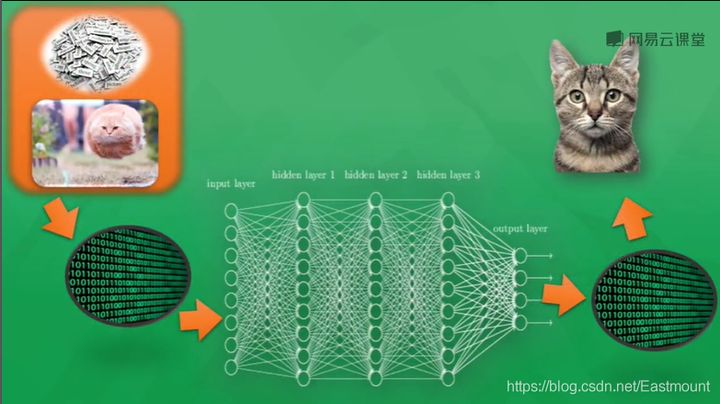
As shown in the figure above, generally speaking, the things processed by computers are different from human beings. Whether it is sound, picture or text, they can only appear in the computer neural network as the number 0 or 1. The pictures seen by the neural network are actually a pile of numbers. The processing of numbers finally generates another pile of numbers, which has certain cognitive significance. Through a little processing, we can know whether the computer judges whether the picture is a cat or a dog.
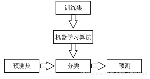
Classification It belongs to supervised learning. It is an important research field in data mining, machine learning and data science. The classification model is similar to human learning. An objective function is obtained by learning the historical data or training set, and then the objective function is used to predict the unknown attributes of the new data set. The classification model mainly includes two steps:
- Training. Given a data set, each sample contains a set of features and a category information, and then the classification algorithm training model is called.
- forecast. The generated model is used to classify and predict the new data set (test set), and judge its classification results.
Usually, in order to test the performance of the learning model, a check set is used. The data set is divided into disjoint training set and test set. The training set is used to construct the classification model, and the test set is used to verify how many class labels are correctly classified.
So what's the difference between regression and classification?
Classification and regression belong to supervised learning. Their difference is that regression is used to predict continuous real values. For example, given the house area to predict the house price, the returned result is the house price; Classification is used to predict limited discrete values, such as judging whether a person is suffering from diabetes, and whether the return value is "yes" or "no". In other words, specify which predefined target class the object belongs to. When the predefined target class is discrete value, it is classification, and when the target class is continuous value, it is regression.
2.MNIST
MNIST is a handwriting recognition data set, which is a very classic example of neural network. MNIST image dataset contains a large number of digital handwritten images, as shown in the figure below. We can try to use it for classification experiments.
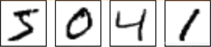
MNIST dataset contains annotation information. The figure above represents numbers 5, 0, 4 and 1 respectively. The dataset consists of three parts:
- Training data set: 55000 samples, mnist.train
- Test data set: 10000 samples, mnist.test
- Validation data set: 5000 samples, mnist.validation
Usually, the training data set is used to train the model, and the verification data set is used to test the correctness and over fitting of the trained model. The test set is invisible (equivalent to a black box), but our ultimate goal is to optimize the effect of the trained model on the test set (here is accuracy).
As shown in the figure below, the data is read by the computer in this form, such as 28 * 28 = 784 pixels. The white places are 0, and the black places indicate numbers. There are 55000 pictures in total.
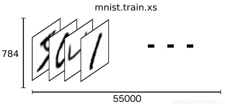
A sample data in MNIST dataset contains two parts: handwritten pictures and corresponding labels. Here, we use xs and ys to represent the picture and the corresponding label respectively. Both the training data set and the test data set have xs and ys. mnist.train.images and mnist.train.labels are used to represent the picture data and the corresponding label data in the training data set.
As shown in the figure below, it represents a picture composed of 2828 pixel matrix. If the number 784 (2828) is placed in our neural network, it is the size of x input. The corresponding matrix is shown in the figure below, and the class label label is 1.
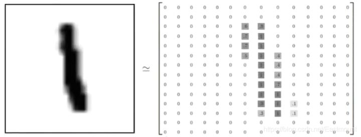
Finally, the training data set of MNIST forms a tensor with a shape of 55000 * 784 bits, that is, a multidimensional array. The first dimension represents the index of the picture, and the second dimension represents the index of the pixels in the picture (the pixel value in the tensor is between 0 and 1).
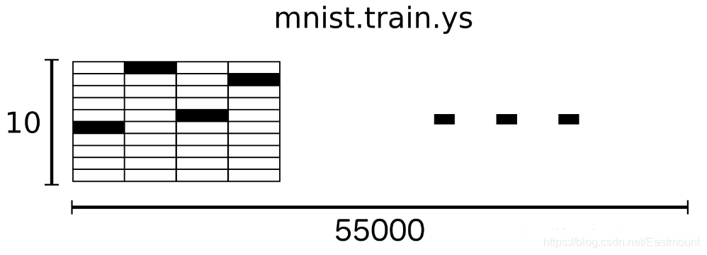
The y value here is actually a matrix. This matrix has 10 positions. If it is 1, it writes 1 at the position of 1 (the second number) and 0 elsewhere; If it is 2, it writes 1 at position 2 (the third number) and 0 at other positions. In this way, the numbers at different positions are classified. For example, the number 3 is represented by [0,0,0,1,0,0,0,0,0], as shown in the following figure.

mnist.train.labels is a 55000 * 10 two-dimensional array, as shown in the figure below. It represents 55000 data points, the first data y represents 5, the second data y represents 0, the third data y represents 4, and the fourth data y represents 1.
Knowing the composition of MNIST dataset and the specific meaning of x and y, let's start writing Keras!
2, Implementation of MNIST classification by Keras
This paper builds a classification neural network through Keras, and then trains MNIST data set. Where X represents a picture, 28 * 28, and y corresponds to the label of the image.
The first step is to import the expansion package.
import numpy as np
from keras.datasets import mnist
from keras.utils import np_utils
from keras.models import Sequential
from keras.layers import Dense, Activation
from keras.optimizers import RMSprop
The second step is to load MNIST data and preprocess.
- X_train.reshape(X_train.shape[0], -1) / 255
Each pixel is standardized and converted from 0-255 to 0-1. - np_utils.to_categorical(y_train, nb_classes=10)
Call up_utils converts the class label into a value of 10 lengths. If the number is 3, it will be marked as 1 in the corresponding place and 0 in other places, that is {0,0,0,1,0,0,0,0}.
Since the MNIST dataset is the sample data of Keras or TensorFlow, we only need the following line of code to read the dataset. If the dataset does not exist, it will be downloaded online. If the dataset has been downloaded, it will be called directly.
# Download MNIST data
# X shape(60000, 28*28) y shape(10000, )
(X_train, y_train), (X_test, y_test) = mnist.load_data()

# Data preprocessing
X_train = X_train.reshape(X_train.shape[0], -1) / 255  # normalize
X_test = X_test.reshape(X_test.shape[0], -1) / 255     # normalize

# Convert the class vector into a class matrix and the number 5 into a 0 0 0 0 0 0 1 0 0 0 0 0 0 0 0 0 matrix
y_train = np_utils.to_categorical(y_train, num_classes=10)
y_test = np_utils.to_categorical(y_test, num_classes=10)
The third step is to create a neural network layer.
The method to create the neural network layer described earlier is to add the neural layer by using add() after definition.
- model = Sequential()
- model.add(Dense(output_dim=1, input_dim=1))
Here, another method is used to add the neural layer through the list when Sequential() is defined. At the same time, it should be noted that the neural network excitation function is added here and RMSprop is called to accelerate the neural network.
- from keras.layers import Dense, Activation
- from keras.optimizers import RMSprop
The neural network layer is:
- The first layer is Dense(32, input_dim=784), which converts the incoming 784 into 32 outputs
- This data loads an excitation function Activation('relu ') and converts it into nonlinear data
- The second layer is Dense(10), which outputs 10 units. At the same time, Keras defines the neural layer, and its input will be the output of the previous layer by default, i.e. 32 (omitted)
- Then, an excitation function Activation('softmax ') is loaded for classification
# Another way to build your neural net
model = Sequential([
        Dense(32, input_dim=784),  # Input value 784 (28 * 28) = > output value 32
        Activation('relu'),        # Conversion of excitation function into nonlinear data
        Dense(10),                 # The output is a result of 10 units
        Activation('softmax')      # The excitation function calls softmax for classification
        ])

# Another way to define your optimizer
rmsprop = RMSprop(lr=0.001, rho=0.9, epsilon=1e-08, decay=0.0) #Learning rate lr

# We add metrics to get more results you want to see
# Activating neural network
model.compile(
        optimizer = rmsprop,                 # Accelerating neural network
        loss = 'categorical_crossentropy',   # loss function
        metrics = ['accuracy'],               # Calculation error or accuracy
        )
The fourth step is neural network training and prediction.
print("Training")
model.fit(X_train, y_train, nb_epoch=2, batch_size=32)    # Training times and size of each batch

print("Testing")
loss, accuracy = model.evaluate(X_test, y_test)

print("loss:", loss)
print("accuracy:", accuracy)
Full code:
# -*- coding: utf-8 -*-
"""
Created on Fri Feb 14 16:43:21 2020
@author: Eastmount CSDN YXZ
O(∩_∩)O Wuhan Fighting!!!
"""
import numpy as np
from keras.datasets import mnist
from keras.utils import np_utils
from keras.models import Sequential
from keras.layers import Dense, Activation
from keras.optimizers import RMSprop
#---------------------------Loading data and preprocessing---------------------------
# Download MNIST data
# X shape(60000, 28*28) y shape(10000, )
(X_train, y_train), (X_test, y_test) = mnist.load_data()
# Data preprocessing
X_train = X_train.reshape(X_train.shape[0], -1) / 255 # normalize
X_test = X_test.reshape(X_test.shape[0], -1) / 255 # normalize
# Convert the class vector into a class matrix and the number 5 into a 0 0 0 0 0 0 1 0 0 0 0 0 0 0 0 0 matrix
y_train = np_utils.to_categorical(y_train, num_classes=10)
y_test = np_utils.to_categorical(y_test, num_classes=10)
#---------------------------Create neural network layer---------------------------
# Another way to build your neural net
model = Sequential([
Dense(32, input_dim=784), # Input value 784 (28 * 28) = > output value 32
Activation('relu'), # Conversion of excitation function into nonlinear data
Dense(10), # The output is a result of 10 units
Activation('softmax') # The excitation function calls softmax for classification
])
# Another way to define your optimizer
rmsprop = RMSprop(lr=0.001, rho=0.9, epsilon=1e-08, decay=0.0) #Learning rate lr
# We add metrics to get more results you want to see
# Activating neural network
model.compile(
optimizer = rmsprop, # Accelerating neural network
loss = 'categorical_crossentropy', # loss function
metrics = ['accuracy'], # Calculation error or accuracy
)
#------------------------------Training and prediction------------------------------
print("Training")
model.fit(X_train, y_train, nb_epoch=2, batch_size=32) # Training times and size of each batch
print("Testing")
loss, accuracy = model.evaluate(X_test, y_test)
print("loss:", loss)
print("accuracy:", accuracy)
Run the code and download it first MNIT Data set.
Using TensorFlow backend.
Downloading data from https://s3.amazonaws.com/img-datasets/mnist.npz
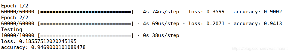
11493376/11490434 [==============================] - 18s 2us/stepThen output the results of two training, we can see that the error is decreasing and the accuracy is increasing. The error loss of the final test output is "0.185575" and the accuracy is "0.94690".
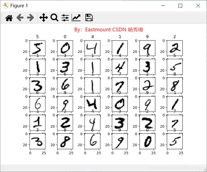
If readers want to more intuitively view the graphics of our digital classification, they can define functions and display them.
The complete code at this time is as follows:
# -*- coding: utf-8 -*-
"""
Created on Fri Feb 14 16:43:21 2020
@author: Eastmount CSDN YXZ
O(∩_∩)O Wuhan Fighting!!!
"""
import numpy as np
from keras.datasets import mnist
from keras.utils import np_utils
from keras.models import Sequential
from keras.layers import Dense, Activation
from keras.optimizers import RMSprop
import matplotlib.pyplot as plt
from PIL import Image

#---------------------------Loading data and preprocessing---------------------------
# Download MNIST data
# X shape(60000, 28*28) y shape(10000, )
(X_train, y_train), (X_test, y_test) = mnist.load_data()

#------------------------------Display picture------------------------------
def show_mnist(train_image, train_labels):
    n = 6
    m = 6
    fig = plt.figure()
    for i in range(n):
        for j in range(m):
            plt.subplot(n,m,i*n+j+1)
            index = i * n + j #Label of the current picture
            img_array = train_image[index]
            img = Image.fromarray(img_array)
            plt.title(train_labels[index])
            plt.imshow(img, cmap='Greys')
    plt.show()

show_mnist(X_train, y_train)

# Data preprocessing
X_train = X_train.reshape(X_train.shape[0], -1) / 255  # normalize
X_test = X_test.reshape(X_test.shape[0], -1) / 255     # normalize

# Convert the class vector into a class matrix and the number 5 into a 0 0 0 0 0 0 1 0 0 0 0 0 0 0 0 0 matrix
y_train = np_utils.to_categorical(y_train, num_classes=10)
y_test = np_utils.to_categorical(y_test, num_classes=10)

#---------------------------Create neural network layer---------------------------
# Another way to build your neural net
model = Sequential([
        Dense(32, input_dim=784),  # Input value 784 (28 * 28) = > output value 32
        Activation('relu'),        # Conversion of excitation function into nonlinear data
        Dense(10),                 # The output is a result of 10 units
        Activation('softmax')      # The excitation function calls softmax for classification
        ])

# Another way to define your optimizer
rmsprop = RMSprop(lr=0.001, rho=0.9, epsilon=1e-08, decay=0.0) #Learning rate lr

# We add metrics to get more results you want to see
# Activating neural network
model.compile(
        optimizer = rmsprop,                 # Accelerating neural network
        loss = 'categorical_crossentropy',   # loss function
        metrics = ['accuracy'],               # Calculation error or accuracy
        )

#------------------------------Training and prediction------------------------------
print("Training")
model.fit(X_train, y_train, nb_epoch=2, batch_size=32)    # Training times and size of each batch
print("Testing")
loss, accuracy = model.evaluate(X_test, y_test)

print("loss:", loss)
print("accuracy:", accuracy)
Click focus to learn about Huawei cloud's new technologies for the first time~