Series articles
- Chapter VIII Teach you hand in hand: Stock Forecasting System Based on LSTM
- Chapter VII Teach you by hand: fruit classification and recognition system based on depth residual network (ResNet)
- Chapter VI Hand in hand teach you: face recognition video coding
1, Project introduction
This paper mainly introduces how to use python to build a personal loan default prediction model based on three classical machine learning algorithms.
The project only uses the prediction of individual loan default as a guide, which contains the relevant code of prediction using the model. The main functions are as follows:
- Data preprocessing.
- Model construction and training, three models: Naive Bayes, random forest and logistic regression.
- Predict the default and evaluate the model.
If you need to replace the training data of children's shoes, you can replace the images and annotation files according to the source code and run them directly.
Bloggers have also referred to articles on the construction of machine learning model, but most of them are theory rather than method. Many students certainly don't need to know much about the principle. They just need to build a prediction system.
This article will only tell you how to quickly build and run a prediction model based on personal loan default. You can refer to other bloggers for principles.
It is precisely because I found that most posts on the Internet only introduce the principle, and the function realization is relatively few.
If you have the above ideas, you'll find the right place!
No more nonsense, go straight to the point!
2, Data set introduction
- We will use the lending data on the lending club, a personal to personal lending website. The lending club provides detailed historical data on successful loans (loans approved by the lending club and co lenders) and failed loans (loans rejected by the lending club and co lenders, and the money has not changed hands).
3, Environmental installation
The IDE developed in this project uses: Jupiter notebook. You can directly search csdn for many installation guides, which will not be repeated here.
Because the project is based on TensorFlow, the following environment is required:
- pandas
- scikit-learn
- numpy
- matplotlib
4, Code introduction
- After the environment is installed, you can start to execute code happily. Due to the large number of codes, the final code will not be put into the blog. Children's shoes in need can be found in [code download address] Download all codes.
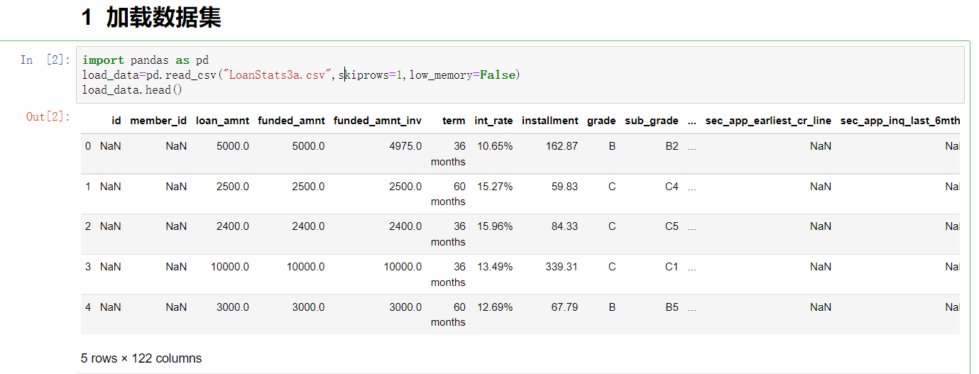
1. Data preprocessing
- First, we will do some feature selection and data cleaning for the read data.
- Field information:
- loan_amnt: Loan
- term: accounting period
- int_rate: international exchange rate
- Installation: installment
- loan_status: Loan Status
- wait
load_data_clean=load_data[['loan_amnt','funded_amnt','term','int_rate',
'installment','emp_length','dti',
'annual_inc','total_pymnt',
'total_pymnt_inv',
'total_rec_int','loan_status']]
del load_data
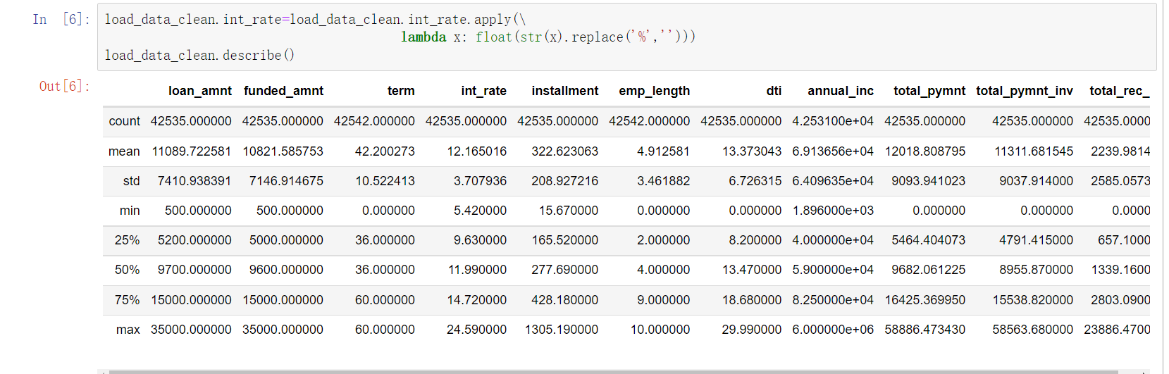
#Note that the input variable must be a quantized value, not a string
#Data cleaning is mainly used to convert data types and deal with missing data
#It is realized by using the function for the elements of the matrix
import re #Regular expression package
def extract_number(string):
num=re.findall('\d+',str(string))
if len(num)>0:
return int(num[0])
else:
return 0;
load_data_clean.emp_length=load_data_clean.emp_length.apply(extract_number)
load_data_clean.head()
- Data after processing:
2. Data visualization exploration
2.1 visualization of features
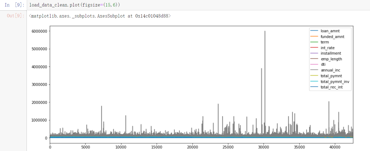
- You can see the annual_ The characteristic fluctuation of Inc is relatively large.
2.2 loan amount
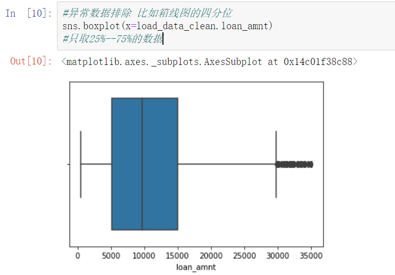
- It can be seen that the loan amount of most people is in the range of 5k-15k.
2.3 relationship between loan amount and installment payment
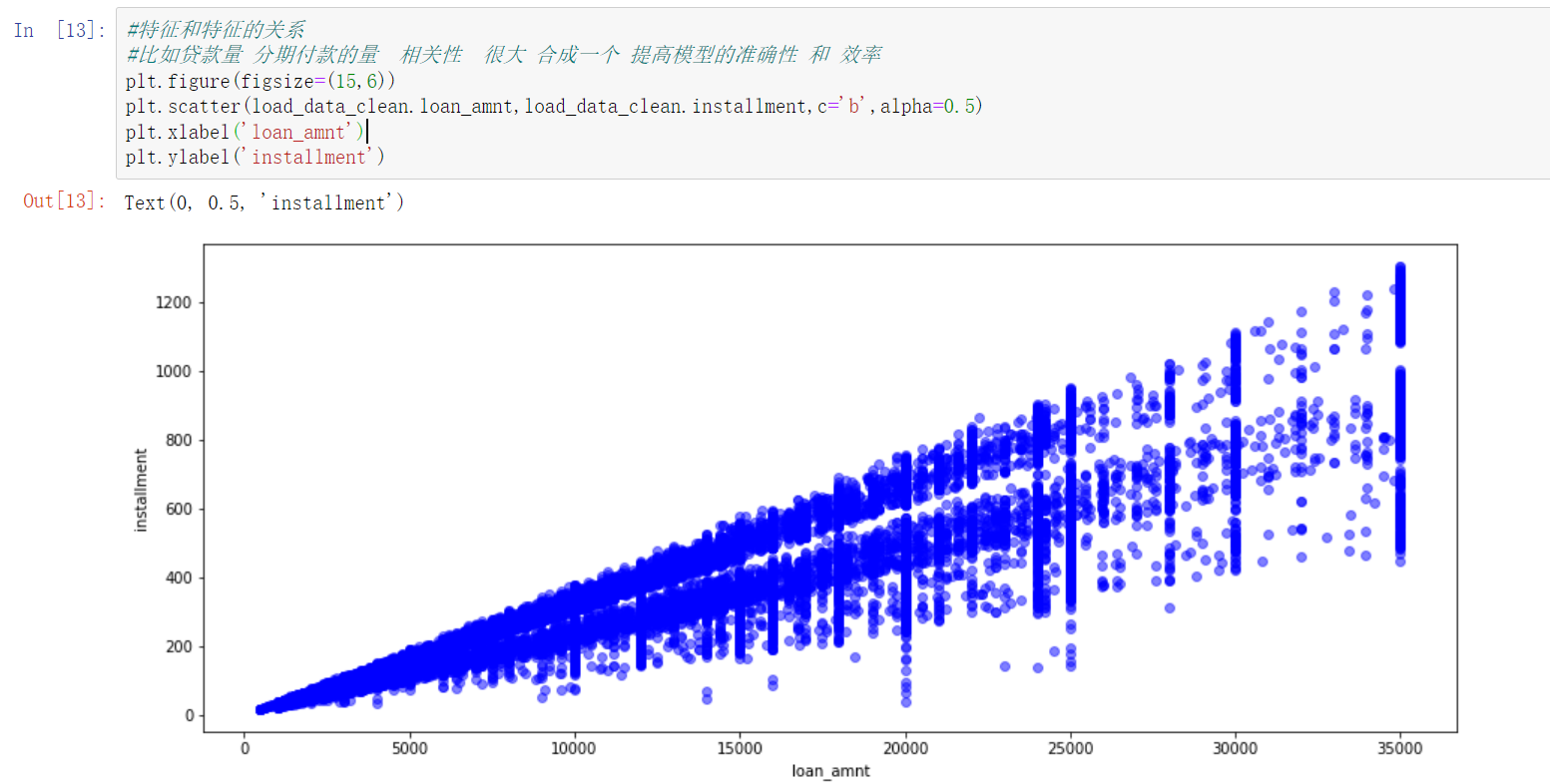
- Here will be: loan_amnt: loan amount; installation: installment amount for correlation analysis.
- It can be seen that loans and installment payments are highly correlated. We can consider combining these two features in the future to improve the accuracy and efficiency of the model.
2.4 whether the loan has been repaid
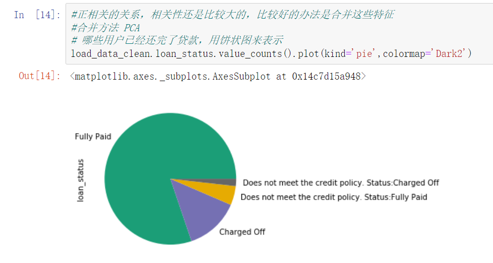
- You can see the ratio of whether the loan is repaid in full and on time in the data.
3. Build model and train
- After the above data processing, we build three different models for training and prediction.
3.1 naive Bayes
- Model and train:
	gnb_model=GaussianNB()
	gnb_model.fit(X_train,Y_train)
 	# Training set
	#Model prediction can give probabilistic results
	train_probs=gnb_model.predict_proba(X_train)
	#Returns the result with the highest probability
	train_predict=gnb_model.predict(X_train)

	# Test set
	#Model prediction can give probabilistic results
	test_probs=gnb_model.predict_proba(X_test)
	#Returns the result with the highest probability
	test_predict=gnb_model.predict(X_test)
- Model prediction score:
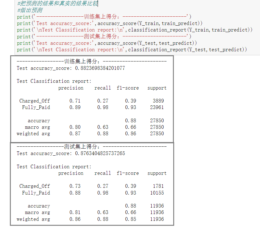
- Let's explain the score of the model. You can see the training set accuracy_score: 0.88. Test set accuracy_score: 0.87.
- The Classification report below is the confusion matrix of two different categories, which outputs the accuracy rate, recall rate and F1 score of each category respectively.
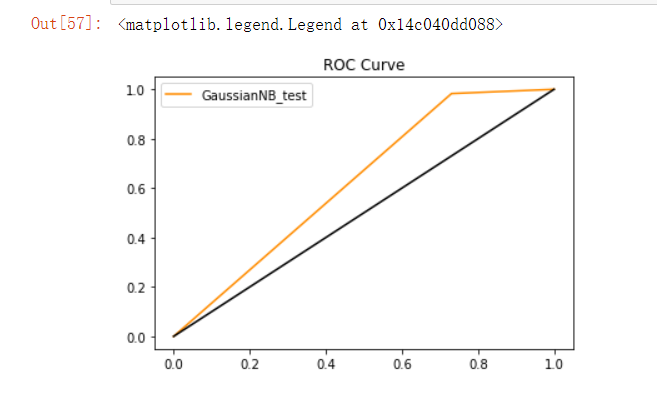
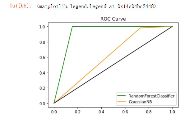
- The ROC curve is as follows:
3.2 random forest
- Model and train:
from sklearn import datasets,svm,metrics,model_selection,preprocessing
from sklearn.ensemble import RandomForestClassifier
from sklearn.model_selection import GridSearchCV
# Instantiated random forest
rfc=RandomForestClassifier()
# Parameter setting
rf_param_grid = {'n_estimators':[100,200,500], 'min_samples_split':[2,3,5,10],
                 'min_samples_leaf':[4,6,10], 'max_depth':[10,50]}
rf_grid = model_selection.GridSearchCV(rfc, rf_param_grid, cv=5, n_jobs=12, verbose=1, scoring='accuracy')
# Training model
rf_grid.fit(X_train, Y_train)
- Model prediction score:
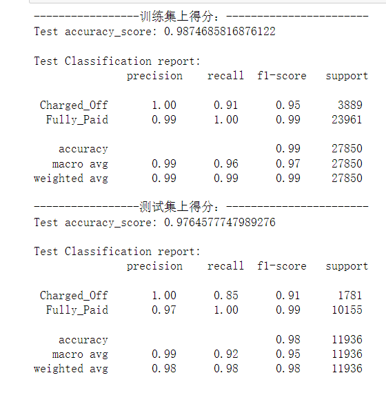
- Similarly, the accuracy score of training set of random forest: 0.987. Test set accuracy score: 0.976
- ROC curves of the above two models:
3.3 logistic regression
- Logistic regression is actually a classification algorithm, so we can also use it to predict whether users may default.
- Model construction and training:
from sklearn.linear_model import LogisticRegression
#Build model parameters
LGR = LogisticRegression(penalty='l2', multi_class='multinomial',solver="newton-cg",n_jobs=12)
# Training model
LGR.fit(X_train, Y_train)
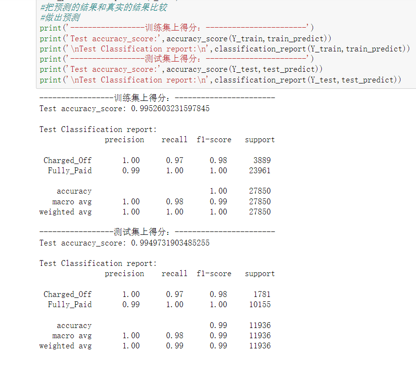
- Model prediction score:
4. Model comparison
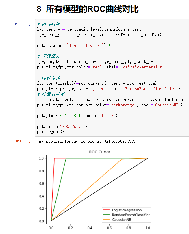
- Because we know that the larger the area occupied by ROC curve, the better the effect of the model will be. According to the above figure, the model effect of red line is the best. Therefore, the application effect of logistic regression model in this data set is the best.
5, Code download address
Due to the large amount of code and data set of the project, interested students can download the code directly. If they encounter any problems in the use process, they can comment in the comment area, and I will answer them one by one.
Code download: