Ten classical sorting algorithms and their optimization
Algorithm overview
0.1 algorithm classification
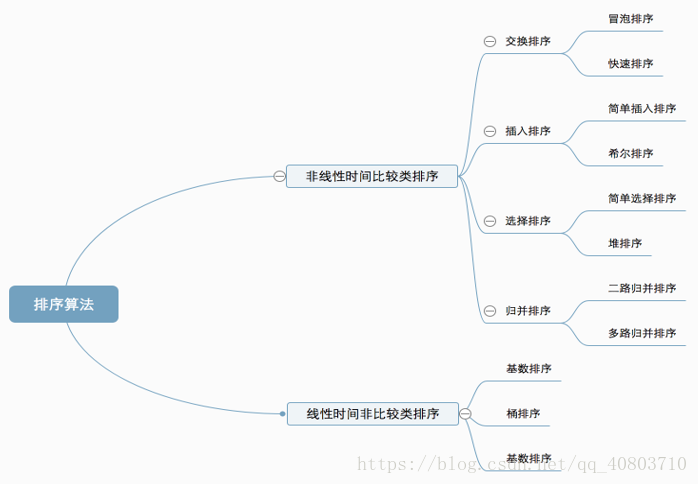
Ten common sorting algorithms can be divided into two categories:
Nonlinear time comparison sort:
The relative order between elements is determined by comparison. Because its time complexity can not exceed O(nlogn), it is called nonlinear time comparison sort.
Including: swap sort (bubble, quick sort), insert sort (simple insert sort, Hill sort), select sort (simple select sort, heap sort) merge sort (two-way, multi-way)
Linear time non comparison sort:
The relative order between elements is determined without comparison, which can break through the lower bound of time based on comparison sorting and run in linear time. Therefore, it is called linear time non comparison sorting.
Including cardinality sorting and bucket sorting
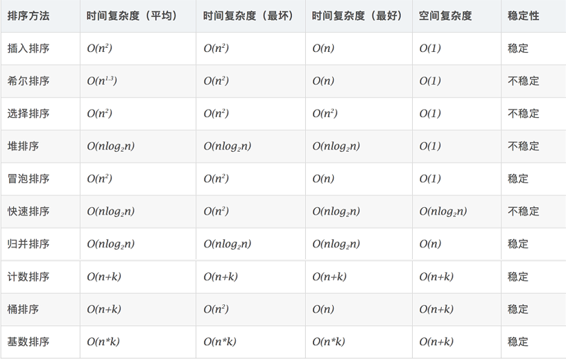
0.2 algorithm complexity
0.3 related concepts
Stable: if a was in front of b and a=b, a will still be in front of b after sorting.
Unstable: if a was originally in front of b and a=b, a may appear after b after sorting.
Time complexity: the total number of operations on sorting data. Reflect the law of operation times when n changes.
Spatial complexity: refers to the measurement of the storage space required for the implementation of the algorithm in the computer. It is also a function of the data scale n.
1. Bubble Sort
Bubble sorting is a simple sorting algorithm. It repeatedly visits the sequence to be sorted, compares two elements at a time, and exchanges them if they are in the wrong order. The work of visiting the sequence is repeated until there is no need to exchange, that is, the sequence has been sorted. The name of this algorithm comes from the fact that smaller elements will slowly "float" to the top of the sequence through exchange.
1.1 algorithm description
- Compare adjacent elements. If the first is bigger than the second, exchange them two;
- Do the same for each pair of adjacent elements, from the first pair at the beginning to the last pair at the end, so that the last element should be the largest number;
- Repeat the above steps for all elements except the last one;
- Repeat steps 1 to 3 until the sorting is completed.
1.2 dynamic diagram demonstration
1.3 code implementation
(1) Optimize 1 (optimize outer loop):
If the exchange of bubble positions is not found in a certain sorting, it indicates that all bubbles in the disordered area to be sorted meet the principle of the lighter is the top and the heavier is the bottom. Therefore, the bubble sorting process can be terminated after this sorting. Therefore, in the algorithm given below, a tag flag is introduced, which is set to 0 before each sorting. If an exchange occurs during sorting, it is set to 1. Check the flag at the end of each sorting. If no exchange has occurred, terminate the algorithm and do not carry out the next sorting.
(2) Optimize 2 (optimize inner loop)
Remember the bubble sort of lastExchange where the last exchange occurred. In each scan, remember the location of lastExchange where the last exchange occurred (the adjacent records after this location have been ordered). At the beginning of the next sorting, R[1... lastExchange-1] is an unordered area and R[lastExchange... n] is an ordered area. In this way, one sort may expand multiple records in the current unordered area, so remember the location of the last exchange lastExchange, so as to reduce the number of sorting trips.
#include<iostream>


using namespace std;


#include<cassert>


//Bubble sorting


void BubbleSort1(int* arr, size_t size)


{


    assert(arr);


    int i = 0, j = 0;


    for (i = 0; i < size - 1; i++)//Sort size-1 times in total


    {


        for (j = 0; j < size - 1 - i; j++)//Select the maximum value of this sort and move back


        {


            if (arr[j] > arr[j + 1])


            {


                int tmp = arr[j];


                arr[j] = arr[j + 1];


                arr[j + 1] = tmp;


            }


        }


    }


}


//Bubble sorting optimization 1


void BubbleSort2(int* arr, size_t size)


{


    assert(arr);


    int i = 0, j = 0;


    for (i = 0; i < size - 1; i++)//Sort size-1 times altogether


    {


        //The flag bit must be set to 0 each time to judge whether the subsequent elements have been exchanged


        int flag = 0;


        for (j = 0; j < size - 1 - i; j++)//Select the maximum value of this sort and move back


        {


            if (arr[j] > arr[j + 1])


            {


                int tmp = arr[j];


                arr[j] = arr[j + 1];


                arr[j + 1] = tmp;


                flag = 1;//As long as there is an exchange, the flag is set to 1


            }


        }


        //Judge whether the flag bit is 0. If it is 0, it means that the following elements are in order. return directly


        if (flag == 0)


        {


            return;


        }


    }


}


//Bubble sorting optimization 2


void BubbleSort3(int* arr, size_t size)


{


    assert(arr);


    int i = 0, j = 0;


    int k = size - 1,pos = 0;   //The pos variable is used to mark the position of the last exchange in the loop


    for (i = 0; i < size - 1; i++)  //Sort size-1 times in total


    {


        //The flag bit must be set to 0 each time to judge whether the subsequent elements have been exchanged


        int flag = 0;


        for (j = 0; j < k; j++)//Select the maximum value of this sort and move back


        {


            if (arr[j] > arr[j + 1])


            {


                int tmp = arr[j];


                arr[j] = arr[j + 1];


                arr[j + 1] = tmp;


                flag = 1;   //As long as there is an exchange, the flag is set to 1


                pos = j;    //The position j of the last exchange in the loop is assigned to pos


            }


        }


        k = pos;


        //Judge whether the flag bit is 0. If it is 0, it means that the following elements are in order. return directly


        if (flag == 0)


        {


            return;


        }


    }


}


int main()


{


    int arr[5] = { 5,4,3,2,1 };


    cout << "The initial sequence is:";


    for (int i = 0; i < 5; i++)


    {


        cout << arr[i] << " ";


    }


    cout << endl;


    /*BubbleSort1(arr, 5);*/


    /*BubbleSort2(arr, 5);*/


    BubbleSort3(arr, 5);


    cout << "The order after bubble sorting is:";


    for (int i = 0; i < 5; i++)


    {


        cout << arr[i] << " ";


    }


    cout << endl;


    system("pause");


    return 0;


}
2. Selection Sort
Selection sort is a simple and intuitive sorting algorithm. Its working principle: first, find the smallest (large) element in the unordered sequence and store it at the beginning of the sorted sequence, then continue to find the smallest (large) element from the remaining unordered elements, and then put it at the end of the sorted sequence. And so on until all elements are sorted.
2.1 algorithm description
For the direct selection sorting of n records, the ordered results can be obtained through n-1 times of direct selection sorting. The specific algorithm is described as follows:
- Initial state: the disordered area is R[1... n], and the ordered area is empty;
- At the beginning of the ith sort (i=1,2,3... n-1), the current ordered area and disordered area are R[1... i-1] and R(i... n) respectively. This sequence selects the record R[k] with the smallest keyword from the current unordered area and exchanges it with the first record r in the unordered area, so that R[1... I] and R[i+1... n) become a new ordered area with an increase in the number of records and a new unordered area with a decrease in the number of records, respectively;
- At the end of n-1 trip, the array is ordered.
2.2 dynamic diagram demonstration
2.3 code implementation
(1) Optimize
Each time you look for the minimum value, you can also find a maximum value, and then place them where they should appear, so that the number of iterations is less. In the code, after the first exchange, if the maximum number was originally placed in the left position, the subscript of the maximum number needs to be restored after the exchange. It should be noted that the subscript of the minimum or maximum value remembered each time is convenient for exchange.
//Select sort


void SelectSort(vector<int>& v)


{


    for(int i = 0; i < v.size() - 2; ++i)


    {


        int k = i;


        for(int j = i + 1; j < v.size() - 1; ++j)


        {


            //Find the subscript of the smallest number


            if(v[j] < v[k])


                k = j;


        }


        if(k != i)


        {


            swap(v[k],v[i]);


        }


    }


}


//optimization


void SelectSort(vector<int>& a)


{


    int left = 0;


    int right = a.size() - 1;


    int min = left;//Store the subscript of the minimum value


    int max = left;//Store the subscript of the maximum value


    while(left <= right)


    {


        min = left;


        max = left;


        for(int i = left; i <= right; ++i)


        {


            if(a[i] < a[min])


            {


                min = i;


            }


            if(a[i] > a[max])


            {


                max = i;


            }


        }


        swap(a[left],a[min]);


        if(left == max)


            max = min;


        swap(a[right],a[max]);


        ++left;


        --right;


    }


}
2.4 algorithm analysis
One of the most stable sorting algorithms, because no matter what data goes in, it is O(n2) time complexity, so when it is used, the smaller the data size, the better. The only advantage may be that it doesn't take up additional memory space. In theory, selective sorting may also be the most common sorting method that most people think of.
3. Insertion Sort
The algorithm description of insertion sort is a simple and intuitive sorting algorithm. Its working principle is to build an ordered sequence, scan the unordered data from back to front in the sorted sequence, find the corresponding position and insert it.
3.1 algorithm description
Generally speaking, insertion sorting is implemented on the array using in place. The specific algorithm is described as follows:
- Starting from the first element, the element can be considered to have been sorted;
- Take out the next element and scan from back to front in the sorted element sequence;
- If the element (sorted) is larger than the new element, move the element to the next position;
- Repeat step 3 until the sorted element is found to be less than or equal to the position of the new element;
- After inserting the new element into this position;
- Repeat steps 2 to 5.
3.2 dynamic diagram demonstration
3.2 code implementation
(1) Optimization 1
Overwrite, merge the two steps of search and data backward. That is, each time a[i] is compared with the previous data a[i-1]. If a[i] > a[i-1], it indicates that a[0... I] is also orderly and does not need to be adjusted. Otherwise, let j=i-1,temp=a[i]. Then search forward while moving the data a[j] backward. When there is data a[j] < a[i], stop and put temp at a[j + 1].
(2) Optimization 2
Then rewrite the method used to insert a[j] into the ordered interval of a[0... j-1], and replace the data backward with data exchange. If a[j] previous data a[j-1] > a[j], exchange a[j] and a[j-1], and then j – until a[j-1] < = a[j]. In this way, a new data can be incorporated into an ordered interval.
//Insert sort


void Insertsort1(int a[], int n)


{


    int i, j, k;


    for (i = 1; i < n; i++)


    {


        //Find a suitable position for a[i] in the previous a[0...i-1] ordered interval


        for (j = i - 1; j >= 0; j--)


            if (a[j] < a[i])


                break;


        //If a suitable position is found


        if (j != i - 1)


        {


            //Move data larger than a[i] backward


            int temp = a[i];


            for (k = i - 1; k > j; k--)


                a[k + 1] = a[k];


            //Place a[i] in the correct position


            a[k + 1] = temp;


        }


    }


}


//Optimization 1


void Insertsort2(int a[], int n)


{


    int i, j;


    for (i = 1; i < n; i++)


        if (a[i] < a[i - 1])


        {


            int temp = a[i];


            for (j = i - 1; j >= 0 && a[j] > temp; j--)


                a[j + 1] = a[j];


            a[j + 1] = temp;


        }


}


//Optimization 2


void Insertsort3(int a[], int n)


{


    int i, j;


    for (i = 1; i < n; i++)


        for (j = i - 1; j >= 0 && a[j] > a[j + 1]; j--)


            Swap(a[j], a[j + 1]);


}
3.4 algorithm analysis
In the implementation of insertion sort, in place sort is usually adopted (that is, the sort that only needs the additional space of O(1)). Therefore, in the process of scanning from back to front, the sorted elements need to be moved back step by step to provide insertion space for the latest elements.
4. Shell Sort
In 1959, Shell invented the first sorting algorithm to break through O(n2), which is an improved version of simple insertion sorting. It differs from insert sort in that it preferentially compares elements that are far away. Hill sort is also called reduced incremental sort.
4.1 algorithm description
First, divide the whole record sequence to be sorted into several subsequences for direct insertion sorting. The specific algorithm description is as follows:
- Select an incremental sequence t1, t2,..., tk, where ti > TJ, tk=1;
- Sort the sequence k times according to the number of incremental sequences k;
- For each sorting, the sequence to be sorted is divided into several subsequences with length m according to the corresponding increment ti, and each sub table is directly inserted and sorted. Only when the increment factor is 1, the whole sequence is treated as a table, and the table length is the length of the whole sequence.
4.2 dynamic diagram demonstration
4.3 code implementation
(1) Optimization 1
Although shellsort1 code is helpful for intuitive understanding of hill sorting, the amount of code is too large and not concise and clear enough. Therefore, make improvements and optimizations. Take the second sorting as an example. It used to start from 1A to 1E and from 2A to 2E each time. It can be changed to start from 1B, first compare with 1A, then take 2B to compare with 2A, and then take 1C to compare with the data in the previous group. This method starts from the gap element of the array every time, and each element is directly inserted and sorted with the data in its own group. Obviously, it is also correct.
(2) Optimization 2
The direct insertion sort part is changed by the third method of direct insertion sort
//Shell Sort


void shellsort1(int a[], int n)


{


    int i, j, gap;


    for (gap = n / 2; gap > 0; gap /= 2) //step


        for (i = 0; i < gap; i++)        //Direct insert sort


        {


            for (j = i + gap; j < n; j += gap)


                if (a[j] < a[j - gap])


                {


                    int temp = a[j];


                    int k = j - gap;


                    while (k >= 0 && a[k] > temp)


                    {


                        a[k + gap] = a[k];


                        k -= gap;


                    }


                    a[k + gap] = temp;


                }


        }


}


//Optimization 1


void shellsort2(int a[], int n)


{


    int j, gap;


    for (gap = n / 2; gap > 0; gap /= 2)


        for (j = gap; j < n; j++)//Start with the gap element of the array


            if (a[j] < a[j - gap])//Each element is directly inserted and sorted with the data in its own group


            {


                int temp = a[j];


                int k = j - gap;


                while (k >= 0 && a[k] > temp)


                {


                    a[k + gap] = a[k];


                    k -= gap;


                }


                a[k + gap] = temp;


            }


}


//Optimization 2


void shellsort3(int a[], int n)


{


    int i, j, gap;


    for (gap = n / 2; gap > 0; gap /= 2)


        for (i = gap; i < n; i++)


            for (j = i - gap; j >= 0 && a[j] > a[j + gap]; j -= gap)


                Swap(a[j], a[j + gap]);


}
4.4 algorithm analysis
The core of Hill sort is the setting of interval sequence. The interval sequence can be set in advance or defined dynamically.
5. Merge Sort
Merge sort is an effective sort algorithm based on merge operation. The algorithm is a very typical application of Divide and Conquer. The ordered subsequences are combined to obtain a completely ordered sequence; That is, each subsequence is ordered first, and then the subsequence segments are ordered. If two ordered tables are merged into one ordered table, it is called 2-way merging.
5.1 algorithm description
- The input sequence with length n is divided into two subsequences with length n/2;
- The two subsequences are sorted by merging;
- Merge two sorted subsequences into a final sorting sequence.
5.2 dynamic diagram demonstration

5.3 code implementation
void mergeArray(int arr[], int first, int mid, int last, int temp[])


{


	int i = first;   //First sequence start position


	int j = mid + 1; //Second sequence start position


	int m = mid;     //First sequence end position


	int n = last;    //Second sequence end position


	int k = 0;       //temp subscript


	while (i <= m && j <= n)  //Is sequence one and two finished


	{


		if (arr[i] < arr[j])  //k always + +, i,j, there is only one at any time++


			temp[k++] = arr[i++];


		else


			temp[k++] = arr[j++];


	}


	while (i <= m)  //Is sequence 1 finished


	{


		temp[k++] = arr[i++];


	}


	while (i <= m && j <= n)  //Is sequence one and two finished


	{


		temp[k++] = arr[j++];


	}


	//Merge into an ordered sequence


	for (i = 0; i < k; i++)


	{


		arr[first + i] = temp[i];


	}


}


void merge(int arr[], int first, int mid, int last, int temp[])


{


	int mid;


	if (first >= last)


		return;


	mid = (first + last) / 2;


	merge(arr,first,mid,temp);


	merge(arr, mid+1, last, temp);


	mergeArray(arr, first, mid,last,temp);


}


void mergeSort(int arr[], int num)


{


	int *temp = (int *)malloc(sizeof(arr[0])*num);


	if (temp == NULL)


		return;


	merge(arr, 0, num - 1, temp);


}
5.4 algorithm analysis
Merge sort is a stable sort method. Like selective sorting, the performance of merge sorting is not affected by the input data, but it is much better than selective sorting, because it is always O(nlogn) time complexity. The cost is the need for additional memory space.
6. Quick Sort
Basic idea of quick sort: divide the records to be arranged into two independent parts through one-time sorting. If the keywords of one part of the records are smaller than those of the other part, the records of the two parts can be sorted separately to achieve the order of the whole sequence.
6.1 algorithm description
Quick sort uses divide and conquer to divide a list into two sub lists. The specific algorithm is described as follows:
- Pick out an element from the sequence, which is called "pivot";
- Reorder the sequence. All elements smaller than the benchmark value are placed in front of the benchmark, and all elements larger than the benchmark value are placed behind the benchmark (the same number can be on either side). After the partition exits, the benchmark is in the middle of the sequence. This is called a partition operation;
- Recursively sorts subsequences that are smaller than the reference value element and subsequences that are larger than the reference value element.
6.2 dynamic diagram demonstration
6.3 code implementation
int QKPass(int r[], int left, int right)


{


	int low = left;


	int high = right;


	r[0] = r[left];


	while (low < high)


	{


		while (low < high && r[high] > r[0])


		{


			high--;


		}


		if (low < high)


		{


			r[low] = r[high];


			low++;


		}


		while (low < high && r[low] < r[0])


		{


			low++;


		}


		if (low < high)


		{


			r[high] = r[low];


			high--;


		}


	}


	r[low] = r[0];


	return low;


}


void QKSort(int r[], int low,int high)


{


	if (low < high)


	{


		int pos = QKPass(r,low,high);


		QKSort(r, low, pos - 1);


		QKSort(r, pos + 1, high);


	}


}
Optimization 1: three average partition method
Select the middle value of the leftmost, rightmost and middle elements of the array to be arranged as the central axis. The median value is selected by comparison. The advantage of taking these three values is that in practical problems, the probability of approximate sequential data or reverse sequential data is large. At this time, the intermediate data must become the median, which is also the approximate median in fact. In case of encountering data that is just large in the middle and small on both sides (or vice versa), the values taken are close to the maximum value, the actual efficiency will increase by about twice because the two parts can be separated at least, which is conducive to slightly disrupting the data and damaging the degraded structure.
When the data set is small, it is not necessary to call the quick sorting algorithm recursively, but call other sorting algorithms with strong processing ability for small-scale data sets. Introport is such an algorithm. It starts to use the quick sort algorithm for sorting. When the recursion reaches a certain depth, it is changed to heap sorting. It overcomes the complex axis selection of quick sort in small-scale data set processing, and also ensures the complexity of heap sort in the worst case O(n log n).
//Implementation of introort algorithm


//The dividing line of data volume determines whether quick sort/heap sort or insertion sort is used


const int threshold=16;


//Auxiliary functions used for heap sorting


int parent(int i)


{


    return (int)((i-1)/2);


}


int left(int i)


{


    return 2 * i+1;


}


int right(int i)


{


    return (2 * i + 2);


}


void heapShiftDown(int heap[], int i, int begin,int end)


{


    int l = left(i-begin)+begin;


    int r = right(i-begin)+begin;


    int largest=i;


	//Find the largest between the left and right word nodes and the parent node


    if(l < end && heap[l] > heap[largest])


        largest = l;


    if(r < end && heap[r] > heap[largest])


        largest = r;


	//If the largest is not the parent node, you need to exchange data and continue scrolling down to meet the maximum heap characteristics


    if(largest != i)


    {


		swap(heap[largest],heap[i]);


        heapShiftDown(heap, largest, begin,end);


    }


}


 //Build the heap from the bottom up, that is, from the penultimate layer of the heap


void buildHeap(int heap[],int begin,int end)


{


    for(int i = (begin+end)/2; i >= begin; i--)


    {


        heapShiftDown(heap, i, begin,end);


    }


}


 //Heap sort


void heapSort(int heap[], int begin,int end)


{


    buildHeap(heap,begin,end);


    for(int i = end; i >begin; i--)


    {


		swap(heap[begin],heap[i]);


        heapShiftDown(heap,begin,begin, i);


    }


}


//Insert sort


void insertionSort(int array[],int len)


{


    int i,j,temp;


    for(i=1;i<len;i++)


    {


      temp = array[i];//store the original sorted array in temp


      for(j=i;j>0 && temp < array[j-1];j--)//compare the new array with temp(maybe -1?)


      {


          array[j]=array[j-1];//all larger elements are moved one pot to the right


      }


      array[j]=temp;


    }


}


//Three point median


int median3(int array[],int first,int median,int end)


{


		if(array[first]<array[median])


		{


				if(array[median]<array[end])


						return median;


				else if(array[first]<array[end])


						return end;


				else


						return first;


		}


		else if(array[first]<array[end])


				return first;


		else if(array[median]<array[end])


				return end;


		else


				return median;


}


//Split array


int partition(int array[],int left,int right,int p)


{


		//Select the rightmost element as the division criteria


		int index = left;


		swap(array[p],array[right]);


		int pivot = array[right];


	    //Move all points smaller than the standard to the left of the index


        for (int i=left; i<right; i++)


        {


                if (array[i] < pivot)


                        swap(array[index++],array[i]);


        }


		//Exchange the standard with the element pointed to by index and return index, that is, the split position


        swap(array[right],array[index]);


        return index;


}


//Recursively split and sort the array


void introSortLoop(int array[],int begin,int end,int depthLimit)


{


		while((end-begin+1)>threshold) //The data size of the subarray is handled by the subsequent insertion sort


		{


				if(depthLimit==0)      //If the recursion depth is too large, heap sorting is used instead


				{


						heapSort(array,begin,end);


						return ;


				}


				--depthLimit;


				//Sort using quick sort


				int cut=partition(array,begin,end,


								median3(array,begin,begin+(end-begin)/2,end));


				introSortLoop(array,cut,end,depthLimit);


				end=cut;    //sort recursively for the left half


		}


}


//Calculate the maximum allowable recursion depth


int lg(int n)


{


		int k;


		for(k=0;n>1;n>>=1) ++k;


		return k;


}


//Domineering introort


void introSort(int array[],int len)


{


		if(len!=1)


		{


				introSortLoop(array,0,len-1,lg(len)*2);


				insertionSort(array,len);


		}


}
Optimization 2: stop the quick sort algorithm when the size of the partition reaches a certain hour. That is, the final product of the quick sorting algorithm is an ordered sequence with "almost" sorting. Some elements in the sequence are not arranged in the final ordered sequence, but there are not many such elements. The "almost" sorted sequence can be sorted by using the insertion sorting algorithm to finally complete the whole sorting process. Because insertion sort has nearly linear complexity for this sort sequence that is "almost" completed. This improvement is proved to be much more effective than the continuous use of fast sorting algorithm.
Optimization 3: when recursively sorting sub partitions, always choose the smallest partition to prioritize. This choice can make more effective use of storage space, so as to speed up the implementation of the algorithm as a whole.
For the quick sort algorithm, in fact, a lot of time is consumed in the partition. Especially when the values of all elements to be partitioned are equal, the general quick sort algorithm falls into the worst case, that is, repeatedly exchanging the same elements and returning the worst central axis value. One way to improve this situation is to divide the partition into three blocks instead of the original two blocks: one is all elements less than the central axis value, one is all elements equal to the central axis value, and the other is all elements greater than the central axis value. Another simple improvement method is to avoid recursive calls and adopt other sorting algorithms if the values of the leftmost and rightmost elements are found to be equal after the partition is completed.
7. Heap Sort
Heap sort is a sort algorithm designed by using the data structure of heap. Heap is a structure similar to a complete binary tree and satisfies the nature of heap: that is, the key value or index of a child node is always less than (or greater than) its parent node.
7.1 algorithm description
- The initial keyword sequence to be sorted (R1,R2,... Rn) is constructed into a large top heap, which is the initial unordered area;
- Exchange the top element R[1] with the last element R[n], and a new disordered region (R1,R2,... Rn-1) and a new ordered region (Rn) are obtained, and R[1,2... N-1] < = R[n];
- Since the new heap top R[1] may violate the nature of the heap after exchange, it is necessary to adjust the current unordered area (R1,R2,... Rn-1) to a new heap, and then exchange R[1] with the last element of the unordered area again to obtain a new unordered area (R1,R2,... Rn-2) and a new ordered area (Rn-1,Rn). Repeat this process until the number of elements in the ordered area is n-1, and the whole sorting process is completed.
7.2 dynamic diagram demonstration
7.3 code implementation
//Heap sort


void HeapSort(int arr[],int len){


    int i;


    //Initialize the heap, starting with the last parent node


    for(i = len/2 - 1; i >= 0; --i){


        Heapify(arr,i,len);


    }


    //Take the largest element from the heap and adjust the heap


    for(i = len - 1;i > 0;--i){


        int temp = arr[i];


        arr[i] = arr[0];


        arr[0] = temp;


        //Adjust to pile


        Heapify(arr,0,i);


    }


}


Then look at the functions that adjust the heap


void Heapify(int arr[], int first, int end){


    int father = first;


    int son = father * 2 + 1;


    while(son < end){


        if(son + 1 < end && arr[son] < arr[son+1]) ++son;


        //If the parent node is larger than the child node, the adjustment is completed


        if(arr[father] > arr[son]) break;


        else {


         //Otherwise, the elements of the parent and child nodes are exchanged


            int temp = arr[father];


            arr[father] = arr[son];


            arr[son] = temp;


            //The parent and child nodes become the next location to compare


            father = son;


            son = 2 * father + 1;


        }


    }


}
var len;   // Because multiple functions declared need data length, set len as a global variable


function buildMaxHeap(arr) {  // Build large top reactor


    len = arr.length;


    for (var i = Math.floor(len/2); i >= 0; i--) {


        heapify(arr, i);


    }


}


function heapify(arr, i) {    // Heap adjustment


    var left = 2 * i + 1,


        right = 2 * i + 2,


        largest = i;


    if (left < len && arr[left] > arr[largest]) {


        largest = left;


    }


    if (right < len && arr[right] > arr[largest]) {


        largest = right;


    }


    if (largest != i) {


        swap(arr, i, largest);


        heapify(arr, largest);


    }


}


function swap(arr, i, j) {


    var temp = arr[i];


    arr[i] = arr[j];


    arr[j] = temp;


}


function heapSort(arr) {


    buildMaxHeap(arr);


    for (var i = arr.length - 1; i > 0; i--) {


        swap(arr, 0, i);


        len--;


        heapify(arr, 0);


    }


    return arr;


}
8. Counting Sort
Counting sort is not a sort algorithm based on comparison. Its core is to convert the input data values into keys and store them in the additional array space. As a sort with linear time complexity, count sort requires that the input data must be integers with a certain range.
8.1 algorithm description
- Find the largest and smallest elements in the array to be sorted;
- Count the number of occurrences of each element with value i in the array and store it in item i of array C;
- All counts are accumulated (starting from the first element in C, and each item is added to the previous item);
- Reverse fill the target array: put each element i in item C(i) of the new array, and subtract 1 from C(i) for each element.
8.2 dynamic diagram demonstration
8.3 code implementation
function countingSort(arr, maxValue) { var bucket =new Array(maxValue + 1), sortedIndex = 0; arrLen = arr.length, bucketLen = maxValue + 1; for (var i = 0; i < arrLen; i++) { if (!bucket[arr[i]]) { bucket[arr[i]] = 0; } bucket[arr[i]]++; } for (var j = 0; j < bucketLen; j++) { while(bucket[j] > 0) { arr[sortedIndex++] = j; bucket[j]--; } } return arr;}
8.4 algorithm analysis
Counting sorting is a stable sorting algorithm. When the input elements are n integers between 0 and K, the time complexity is O(n+k) and the space complexity is O(n+k), and its sorting speed is faster than any comparison sorting algorithm. When k is not very large and the sequences are concentrated, counting sorting is a very effective sorting algorithm.
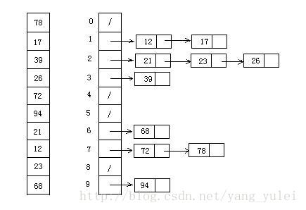
9. Bucket Sort
Bucket sorting is an upgraded version of counting sorting. It makes use of the mapping relationship of the function. The key to efficiency lies in the determination of the mapping function. Working principle of bucket sort: assuming that the input data is uniformly distributed, divide the data into a limited number of buckets, and sort each bucket separately (it is possible to use another sorting algorithm or continue to use bucket sorting recursively).
9.1 algorithm description
- Set a quantitative array as an empty bucket;
- Traverse the input data and put the data into the corresponding bucket one by one;
- Sort each bucket that is not empty;
- Splice the ordered data from a bucket that is not empty.
9.2 picture presentation
9.3 code implementation
function bucketSort(arr, bucketSize) {


    if (arr.length === 0) {


      return arr;


    }


    var i;


    var minValue = arr[0];


    var maxValue = arr[0];


    for (i = 1; i < arr.length; i++) {


      if (arr[i] < minValue) {


          minValue = arr[i];               // Minimum value of input data


      }else if (arr[i] > maxValue) {


          maxValue = arr[i];               // Maximum value of input data


      }


    }


    // Initialization of bucket


    var DEFAULT_BUCKET_SIZE = 5;           // Set the default number of buckets to 5


    bucketSize = bucketSize || DEFAULT_BUCKET_SIZE;


    var bucketCount = Math.floor((maxValue - minValue) / bucketSize) + 1;


    var buckets =new Array(bucketCount);


    for (i = 0; i < buckets.length; i++) {


        buckets[i] = [];


    }


    // The mapping function is used to allocate the data to each bucket


    for (i = 0; i < arr.length; i++) {


        buckets[Math.floor((arr[i] - minValue) / bucketSize)].push(arr[i]);


    }


    arr.length = 0;


    for (i = 0; i < buckets.length; i++) {


        insertionSort(buckets[i]);                     // Sort each bucket. Insert sort is used here


        for (var j = 0; j < buckets[i].length; j++) {


            arr.push(buckets[i][j]);


        }


    }


    return arr;


}
9.4 algorithm analysis
In the best case, the linear time O(n) is used for bucket sorting. The time complexity of bucket sorting depends on the time complexity of sorting the data between buckets, because the time complexity of other parts is O(n). Obviously, the smaller the bucket division, the less data between buckets, and the less time it takes to sort. But the corresponding space consumption will increase.
10. Radix Sort
Cardinality sorting is sorting according to the low order, and then collecting; Then sort according to the high order, and then collect; And so on until the highest position. Sometimes some attributes are prioritized. They are sorted first by low priority and then by high priority. The final order is the high priority, the high priority, the same high priority, and the low priority, the high priority.
10.1 algorithm description
- Get the maximum number in the array and get the number of bits;
- arr is the original array, and each bit is taken from the lowest bit to form a radius array;
- Count and sort the radix (using the characteristics that count sorting is suitable for a small range of numbers);
10.2 dynamic diagram demonstration
10.3 code implementation
// LSD Radix Sort


var counter = [];


function radixSort(arr, maxDigit) {


    var mod = 10;


    var dev = 1;


    for (var i = 0; i < maxDigit; i++, dev *= 10, mod *= 10) {


        for(var j = 0; j < arr.length; j++) {


            var bucket = parseInt((arr[j] % mod) / dev);


            if(counter[bucket]==null) {


                counter[bucket] = [];


            }


            counter[bucket].push(arr[j]);


        }


        var pos = 0;


        for(var j = 0; j < counter.length; j++) {


            var value =null;


            if(counter[j]!=null) {


                while ((value = counter[j].shift()) !=null) {


                      arr[pos++] = value;


                }


          }


        }


    }


    return arr;


}
10.4 algorithm analysis
Cardinality sorting is based on sorting separately and collecting separately, so it is stable. However, the performance of cardinality sorting is slightly worse than bucket sorting. Each bucket allocation of keywords needs O(n) time complexity, and it needs O(n) time complexity to get a new keyword sequence after allocation. If the data to be arranged can be divided into D keywords, the time complexity of cardinality sorting will be O(d*2n). Of course, D is far less than N, so it is basically linear.
The spatial complexity of cardinality sorting is O(n+k), where k is the number of buckets. Generally speaking, n > > k, so about n additional spaces are required.