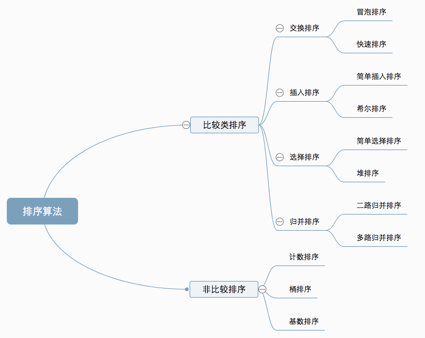
Algorithm overview

Algorithm classification

Ten common sorting algorithms can be divided into two categories:

• Comparison sort: the relative order between elements is determined by comparison. Because its time complexity cannot exceed O(nlogn), it is also called nonlinear time comparison sort.
• Non comparison sort: it does not determine the relative order between elements through comparison. It can break through the time lower bound based on comparison sort and run in linear time. Therefore, it is also called linear time non comparison sort.
  

Algorithm complexity

Related concepts

• Stable: if a was in front of b and a=b, a will still be in front of b after sorting.
• Unstable: if a was originally in front of b and a=b, a may appear after b after sorting.
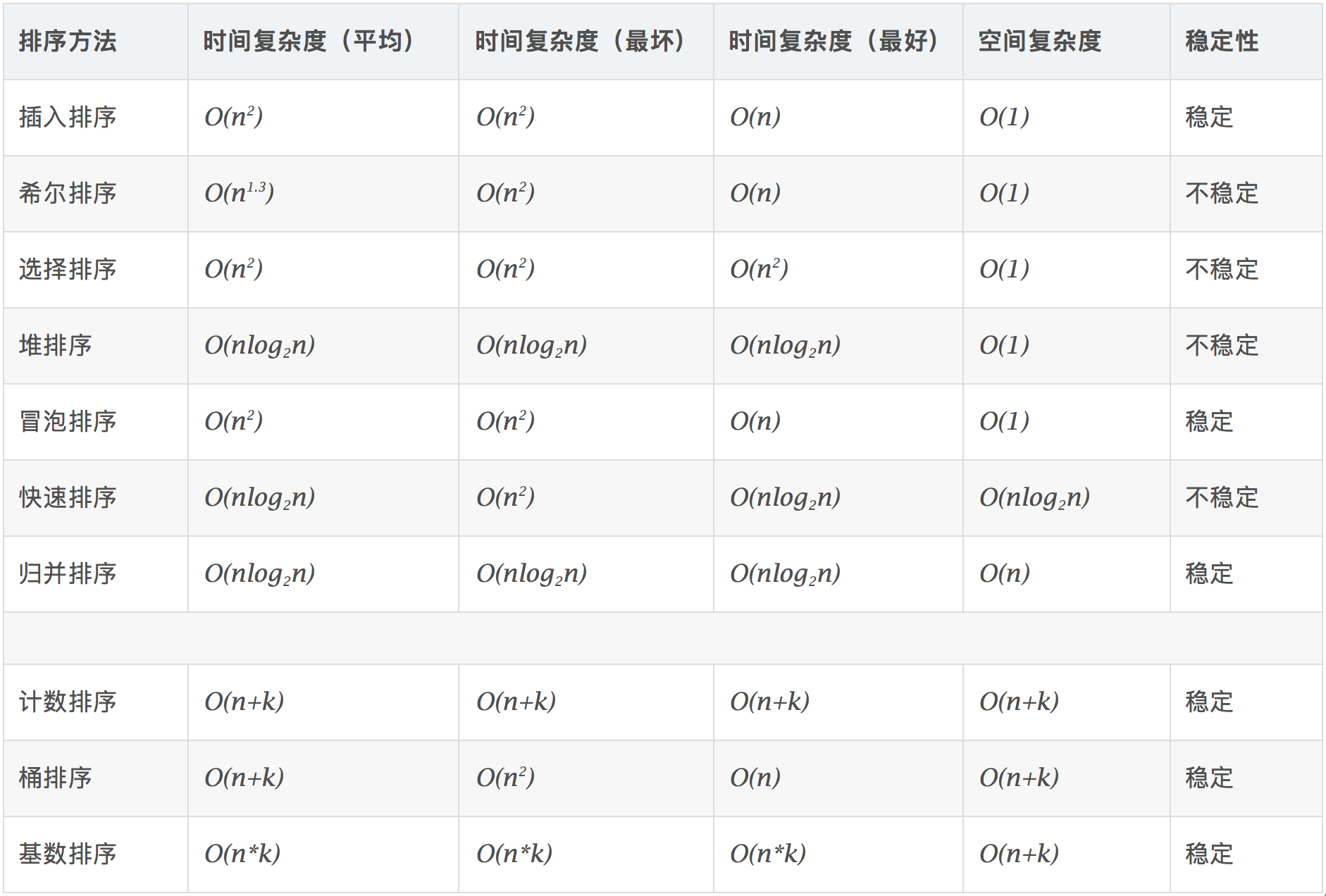
• Time complexity: the total number of operations on sorting data. Reflect the law of operation times when n changes.
• Spatial complexity: refers to the measurement of the storage space required for the implementation of the algorithm in the computer. It is also a function of the data scale n.

1. Bubble Sort

Bubble sorting is a simple sorting algorithm. It repeatedly visits the sequence to be sorted, compares two elements at a time, and exchanges them if they are in the wrong order. The work of visiting the sequence is repeated until there is no need to exchange, that is, the sequence has been sorted. The name of this algorithm comes from the fact that smaller elements will slowly "float" to the top of the sequence through exchange.

Algorithm description

• Compare adjacent elements. If the first is bigger than the second, exchange them two;
• Do the same for each pair of adjacent elements, from the first pair at the beginning to the last pair at the end, so that the last element should be the largest number;
• Repeat the above steps for all elements except the last one;
• Repeat steps 1 to 3 until the sorting is completed.

Dynamic diagram demonstration

code implementation

function bubbleSort(arr) {
    var len = arr.length;
    for(var i = 0; i < len - 1; i++) {
        for(var j = 0; j < len - 1 - i; j++) {
            if(arr[j] > arr[j+1]) {       // Pairwise comparison of adjacent elements
                var temp = arr[j+1];       // Element exchange
                arr[j+1] = arr[j];
                arr[j] = temp;
            }
        }
    }
    return arr;
}

2. Selection Sort

Selection sort is a simple and intuitive sorting algorithm. Its working principle: first find the smallest (large) element in the unordered sequence and store it at the beginning of the sorted sequence, then continue to find the smallest (large) element from the remaining unordered elements, and then put it at the end of the sorted sequence. And so on until all elements are sorted.

Algorithm description

For the direct selection sorting of n records, the ordered results can be obtained through n-1 times of direct selection sorting. The specific algorithm is described as follows:

• Initial state: the disordered region is R[1... n], and the ordered region is empty;
• At the beginning of the i-th sequence (i=1,2,3... n-1), the current ordered area and unordered area are R[1... i-1] and R(i... n) respectively. This sequence selects the record R[k] with the smallest keyword from the current unordered area and exchanges it with the first record R in the unordered area, so that R[1... I] and R[i+1... n) become a new ordered area with an increase in the number of records and a new unordered area with a decrease in the number of records;
• At the end of n-1 trip, the array is ordered.

Dynamic diagram demonstration

code implementation

function selectionSort(arr) {
    var len = arr.length;
    var minIndex, temp;
    for(var i = 0; i < len - 1; i++) {
        minIndex = i;
        for(var j = i + 1; j < len; j++) {
            if(arr[j] < arr[minIndex]) {    // Find the smallest number
                minIndex = j;                // Save the index of the smallest number
            }
        }
        temp = arr[i];
        arr[i] = arr[minIndex];
        arr[minIndex] = temp;
    }
    return arr;
} 

algorithm analysis

One of the most stable sorting algorithms, because no matter what data goes in, it is O(n2) time complexity, so when it is used, the smaller the data size, the better. The only advantage may be that it doesn't take up additional memory space. In theory, selective sorting may also be the most common sorting method that most people think of.

3. Insertion Sort

The algorithm description of insertion sort is a simple and intuitive sorting algorithm. Its working principle is to build an ordered sequence, scan the unordered data from back to front in the sorted sequence, find the corresponding position and insert.

Algorithm description

Generally speaking, insertion sorting is implemented on the array using in place. The specific algorithm is described as follows:

• Starting from the first element, the element can be considered to have been sorted;
• Take out the next element and scan from back to front in the sorted element sequence;
• If the element (sorted) is larger than the new element, move the element to the next position;
• Repeat step 3 until the sorted element is found to be less than or equal to the position of the new element;
• After inserting the new element into this position;
• Repeat steps 2 to 5.

Dynamic diagram demonstration

code implementation

function insertionSort(arr) {
    var len = arr.length;
    var preIndex, current;
    for(var i = 1; i < len; i++) {
        preIndex = i - 1;
        current = arr[i];
        while(preIndex >= 0 && arr[preIndex] > current) {
            arr[preIndex + 1] = arr[preIndex];
            preIndex--;
        }
        arr[preIndex + 1] = current;
    }
    return arr;
}

algorithm analysis

In the implementation of insertion sort, in place sort is usually adopted (i.e. the sort that only needs the additional space of O(1)). Therefore, in the process of scanning from back to front, the sorted elements need to be moved back step by step to provide insertion space for the latest elements.

4. Shell Sort

In 1959, Shell invented the first sorting algorithm to break through O(n2), which is an improved version of simple insertion sorting. It differs from insert sort in that it preferentially compares elements that are far away. Hill sort is also called reduced incremental sort.

Algorithm description

First, divide the whole record sequence to be sorted into several subsequences for direct insertion sorting. The specific algorithm description is as follows:

• Select an incremental sequence t1, t2,..., tk, where ti > TJ, tk=1;
• Sort the sequence k times according to the number of incremental sequences k;
• For each sorting, the sequence to be sorted is divided into several subsequences with length m according to the corresponding increment ti, and each sub table is directly inserted and sorted. Only when the increment factor is 1, the whole sequence is treated as a table, and the table length is the length of the whole sequence.

Dynamic diagram demonstration

code implementation

function shellSort(arr) {
    var len = arr.length;
    for(var gap = Math.floor(len / 2); gap > 0; gap = Math.floor(gap / 2)) {
        // Note: This is different from the dynamic diagram. The dynamic diagram is executed in groups, and the actual operation is that multiple groups are executed alternately
        for(var i = gap; i < len; i++) {
            var j = i;
            var current = arr[i];
            while(j - gap >= 0 && current < arr[j - gap]) {
                 arr[j] = arr[j - gap];
                 j = j - gap;
            }
            arr[j] = current;
        }
    }
    return arr;
}

algorithm analysis

The core of Hill sort is the setting of interval sequence. The interval sequence can be set in advance or defined dynamically. The algorithm for dynamically defining interval sequence was proposed by Robert Sedgewick, co-author of algorithm (4th Edition).

5. Merge Sort

Merge sort is an effective sort algorithm based on merge operation. The algorithm is a very typical application of Divide and Conquer. The ordered subsequences are combined to obtain a completely ordered sequence; that is, each subsequence is ordered first, and then the subsequence segments are ordered. If two ordered tables are combined into one ordered table, it is called 2-way merging.

Algorithm description

• The input sequence with length n is divided into two subsequences with length n/2;
• The two subsequences are sorted by merging;
• Merge two sorted subsequences into a final sorting sequence.

Dynamic diagram demonstration

code implementation

function mergeSort(arr) {
    var len = arr.length;
    if(len < 2) {
        return arr;
    }
    var middle = Math.floor(len / 2),
        left = arr.slice(0, middle),
        right = arr.slice(middle);
    return merge(mergeSort(left), mergeSort(right));
}
 
function merge(left, right) {
    var result = [];
 
    while(left.length>0 && right.length>0) {
        if(left[0] <= right[0]) {
            result.push(left.shift());
        }else{
            result.push(right.shift());
        }
    }
 
    while(left.length)
        result.push(left.shift());
 
    while(right.length)
        result.push(right.shift());
 
    return result;
}

algorithm analysis

Merge sort is a stable sort method. Like the selective sort, the performance of merge sort is not affected by the input data, but it performs much better than the selective sort, because it is always O(nlogn) time complexity. The cost is the need for additional memory space.

6. Quick Sort

Basic idea of quick sort: divide the records to be arranged into two independent parts through one-time sorting. If the keywords of one part of the records are smaller than those of the other part, the records of the two parts can be sorted separately to achieve the order of the whole sequence.

Algorithm description

Quick sort uses divide and conquer to divide a list into two sub lists. The specific algorithm is described as follows:

• Pick out an element from the sequence, which is called "pivot";
• Reorder the sequence. All elements smaller than the benchmark value are placed in front of the benchmark, and all elements larger than the benchmark value are placed behind the benchmark (the same number can be on either side). After this partition exit, the benchmark is in the middle of the sequence. This is called partition operation;
• Recursively sorts subsequences that are smaller than the reference value element and subsequences that are larger than the reference value element.

Dynamic diagram demonstration

code implementation

function quickSort(arr, left, right) {
    var len = arr.length,
        partitionIndex,
        left = typeof left != 'number'? 0 : left,
        right = typeof right != 'number'? len - 1 : right;
 
    if(left < right) {
        partitionIndex = partition(arr, left, right);
        quickSort(arr, left, partitionIndex-1);
        quickSort(arr, partitionIndex+1, right);
    }
    return arr;
}
 
function partition(arr, left ,right) {    // Partition operation
    var pivot = left,                     // Set reference value (pivot)
        index = pivot + 1;
    for(var i = index; i <= right; i++) {
        if(arr[i] < arr[pivot]) {
            swap(arr, i, index);
            index++;
        }       
    }
    swap(arr, pivot, index - 1);
    return index-1;
}
 
function swap(arr, i, j) {
    var temp = arr[i];
    arr[i] = arr[j];
    arr[j] = temp;
}

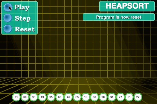
7. Heap Sort

Heap sort is a sort algorithm designed by using heap as a data structure. Heap is a structure similar to a complete binary tree and meets the nature of heap: that is, the key value or index of a child node is always less than (or greater than) its parent node.

Algorithm description

• The initial keyword sequence to be sorted (R1,R2,... Rn) is constructed into a large top heap, which is the initial unordered area;
• Exchange the top element R[1] with the last element R[n], and a new disordered region (R1,R2,... Rn-1) and a new ordered region (Rn) are obtained, and R[1,2... N-1] < = R[n];
• Since the new heap top R[1] may violate the nature of the heap after exchange, it is necessary to adjust the current unordered area (R1,R2,... Rn-1) to a new heap, and then exchange R[1] with the last element of the unordered area again to obtain a new unordered area (R1,R2,... Rn-2) and a new ordered area (Rn-1,Rn). Repeat this process until the number of elements in the ordered area is n-1, and the whole sorting process is completed.

Dynamic diagram demonstration

code implementation

var len;   // Because multiple functions declared need data length, set len as a global variable
 
function buildMaxHeap(arr) {  // Build large top reactor
    len = arr.length;
    for(var i = Math.floor(len/2); i >= 0; i--) {
        heapify(arr, i);
    }
}
 
function heapify(arr, i) {    // Heap adjustment
    var left = 2 * i + 1,
        right = 2 * i + 2,
        largest = i;
 
    if(left < len && arr[left] > arr[largest]) {
        largest = left;
    }
 
    if(right < len && arr[right] > arr[largest]) {
        largest = right;
    }
 
    if(largest != i) {
        swap(arr, i, largest);
        heapify(arr, largest);
    }
}
 
function swap(arr, i, j) {
    var temp = arr[i];
    arr[i] = arr[j];
    arr[j] = temp;
}
 
function heapSort(arr) {
    buildMaxHeap(arr);
 
    for(var i = arr.length - 1; i > 0; i--) {
        swap(arr, 0, i);
        len--;
        heapify(arr, 0);
    }
    return arr;
}

8. Counting Sort

Counting sort is not a sort algorithm based on comparison. Its core is to convert the input data values into keys and store them in the additional array space. As a sort with linear time complexity, count sort requires that the input data must be integers with a certain range.

Algorithm description

• Find the largest and smallest elements in the array to be sorted;
• Count the number of occurrences of each element with value i in the array and store it in item i of array C;
• All counts are accumulated (starting from the first element in C, and each item is added to the previous item);
• Reverse fill the target array: put each element i in item C(i) of the new array, and subtract 1 from C(i) for each element.

Dynamic diagram demonstration

code implementation

function countingSort(arr, maxValue) {
    var bucket = new Array(maxValue + 1),
        sortedIndex = 0;
        arrLen = arr.length,
        bucketLen = maxValue + 1;
 
    for(var i = 0; i < arrLen; i++) {
        if(!bucket[arr[i]]) {
            bucket[arr[i]] = 0;
        }
        bucket[arr[i]]++;
    }
 
    for(var j = 0; j < bucketLen; j++) {
        while(bucket[j] > 0) {
            arr[sortedIndex++] = j;
            bucket[j]--;
        }
    }
 
    return arr;
}

algorithm analysis

Counting sorting is a stable sorting algorithm. When the input elements are n integers between 0 and K, the time complexity is O(n+k) and the space complexity is O(n+k), and its sorting speed is faster than any comparison sorting algorithm. When k is not very large and the sequences are concentrated, counting sorting is a very effective sorting algorithm.

9. Bucket Sort

Bucket sorting is an upgraded version of counting sorting. It makes use of the mapping relationship of the function. The key to efficiency lies in the determination of the mapping function. Working principle of bucket sort: assuming that the input data is uniformly distributed, divide the data into a limited number of buckets, and sort each bucket separately (it is possible to use another sorting algorithm or continue to use bucket sorting recursively).

Algorithm description

• Set a quantitative array as an empty bucket;
• Traverse the input data and put the data into the corresponding bucket one by one;
• Sort each bucket that is not empty;
• Splice the ordered data from a bucket that is not empty.

Dynamic diagram demonstration

code implementation

function bucketSort(arr, bucketSize) {
    if(arr.length === 0) {
      return arr;
    }
 
    var i;
    var minValue = arr[0];
    var maxValue = arr[0];
    for(i = 1; i < arr.length; i++) {
      if(arr[i] < minValue) {
          minValue = arr[i];               // Minimum value of input data
      }else if(arr[i] > maxValue) {
          maxValue = arr[i];               // Maximum value of input data
      }
    }
 
    // Initialization of bucket
    var DEFAULT_BUCKET_SIZE = 5;           // Set the default number of buckets to 5
    bucketSize = bucketSize || DEFAULT_BUCKET_SIZE;
    var bucketCount = Math.floor((maxValue - minValue) / bucketSize) + 1;  
    var buckets = new Array(bucketCount);
    for(i = 0; i < buckets.length; i++) {
        buckets[i] = [];
    }
 
    // The mapping function is used to allocate the data to each bucket
    for(i = 0; i < arr.length; i++) {
        buckets[Math.floor((arr[i] - minValue) / bucketSize)].push(arr[i]);
    }
 
    arr.length = 0;
    for(i = 0; i < buckets.length; i++) {
        insertionSort(buckets[i]);                     // Sort each bucket. Insert sort is used here
        for(var j = 0; j < buckets[i].length; j++) {
            arr.push(buckets[i][j]);                     
        }
    }
 
    return arr;
}

algorithm analysis

In the best case, the linear time O(n) is used for bucket sorting. The time complexity of bucket sorting depends on the time complexity of sorting the data between buckets, because the time complexity of other parts is O(n). Obviously, the smaller the bucket division, the less data between buckets, and the less time it takes to sort. But the corresponding space consumption will increase.

10. Radix Sort

Cardinality sorting is sorting according to the low order, and then collecting; Then sort according to the high order, and then collect; And so on until the highest order. Sometimes some attributes are prioritized. They are sorted first by low priority and then by high priority. The final order is the high priority, the high priority, the same high priority, and the low priority, the high priority.

Algorithm description

• Get the maximum number in the array and get the number of bits;
• arr is the original array, and each bit is taken from the lowest bit to form a radius array;
• Count and sort the radix (using the characteristics that count sorting is suitable for a small range of numbers);

Dynamic diagram demonstration

code implementation

varcounter = [];
function radixSort(arr, maxDigit) {
    var mod = 10;
    var dev = 1;
    for(var i = 0; i < maxDigit; i++, dev *= 10, mod *= 10) {
        for(var j = 0; j < arr.length; j++) {
            var bucket = parseInt((arr[j] % mod) / dev);
            if(counter[bucket]==null) {
                counter[bucket] = [];
            }
            counter[bucket].push(arr[j]);
        }
        var pos = 0;
        for(var j = 0; j < counter.length; j++) {
            var value =null;
            if(counter[j]!=null) {
                while((value = counter[j].shift()) !=null) {
                      arr[pos++] = value;
                }
          }
        }
    }
    return arr;
}

algorithm analysis

Cardinality sorting is based on sorting separately and collecting separately, so it is stable. However, the performance of cardinality sorting is slightly worse than bucket sorting. Each bucket allocation of keywords needs O(n) time complexity, and it needs O(n) time complexity to get a new keyword sequence after allocation. If the data to be sorted can be divided into D keywords, the time complexity of cardinality sorting will be O(d*2n). Of course, D is much less than N, so it is basically linear.

The spatial complexity of cardinality sorting is O(n+k), where k is the number of buckets. Generally speaking, n > > k, so about n additional spaces are required.

Article source: link