Copyright Statement: This article is the original article of the blogger. The source of reprinting should be indicated.
AlexNet
AlexNet was introduced in 2012, and it won the ILSCRC championship in 2012 by a significant margin.
AlexNet applies the basic principles of CNN to deeper networks and adds some new technologies:
1. ReLU is used as the activation function of CNN, which proves that it outperforms Sigmoid in deeper networks.
2. Dropout is used to randomly ignore some neurons in training network to prevent model over-fitting, mainly in the full connection layer.
3. Maximum pooling of overlap is used in CNN. AlexNet uses maximum pooling to avoid ambiguity caused by average pooling. Overlapping is that the size of pooling core is larger than the step of core movement, resulting in overlap and coverage between pooling outputs. Enhancing the richness of features.
4. Using LRN layer to imitate the side inhibition mechanism of biological nervous system is more useful for ReLU, an activation function without upper bound, because it can select larger feedback from the response of several convolution cores nearby to suppress smaller feedback. It is not suitable for Sigmoid, an activation function with fixed boundaries.
5. Use GPU to speed up network training (AlexNet uses two GTX 580)
6. Data enhancement, random image interception, fixed size (224x224), inversion, translation and so on, adding some noise, expanding training data, alleviating over-fitting of the model, and improving generalization ability. In the process of prediction, it is to take the four corners and the middle position of the picture, carry out data enhancement processing, obtain 10 pictures, respectively, to predict and calculate the average of the results. AlexNet's paper also mentioned. By then, the error rate can be reduced by 1% by adding 0.1 Gauss noise to the principal component of the image processed by the RGB data process PCA.

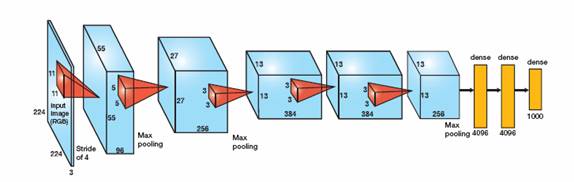
AlexNet's network structure:
1. First, the input layer
2,Conv 11x11,96, Step 4,ReLU
3,LRN(local response norm)
4,max_pool(3x3), step 2
5, Conv 5x5, 256, Step 1,ReLU
6,LRN
7,max_pool(3x3), step 2
8, Conv 3x3, 384, Step 1,ReLU
9,max_pool(3x3), step 2
10,Conv 3x3,384, Step 1,ReLU
11.max_pool(3x3), step 2
12,Conv 3x3,256, Step 1,ReLU
13,max_pool(3x3), step 2
14,FC(fullconnection) 4096,ReLU
15,FC,4096,ReLU
16,FC,1000
ImageNet data sets are huge, AlexNet is very time-consuming, so we still use MNIST to test. Because MNIST is a 28-size image, we can change the size of the network, and omit some LRN operations. The effect of LRN is not particularly obvious, and it will affect the speed of network training. The overall structure is still in accordance with AlexNet. See if we can improve the accuracy.
tensorflow version 1.1, some functions of the parameters of the detailed annotations, reference This simple CNN
import tensorflow as tf
import matplotlib.pyplot as plt
import numpy as np
import time
from tensorflow.examples.tutorials.mnist import input_data
Network parameters
#Defining network hyperparameters
learning_rate = 0.0001
train_epochs = 130
batch_size = 256
display = 10
t = 50      # Number of random sampling per round
# Network parameters
n_input = 784
n_classes = 10
dropout = 0.75     # dropout rule, preserving the probability of neuron nodes
# Define placeholders
images = tf.placeholder(tf.float32,[None,n_input])
labels = tf.placeholder(tf.float32,[None,n_classes])
keep_prob = tf.placeholder(tf.float32)A series of auxiliary functions
# Random sampling of training data
# Random Selection of mini_batch
def get_random_batchdata(n_samples, batchsize):
    start_index = np.random.randint(0, n_samples - batchsize)
    return (start_index, start_index + batchsize)
# Weight, bias initialization
# In the convolution layer and the full connection layer, I use different initialization operations.
# Convolution layer is initialized with truncated orthodox distribution, shape is a list object
def conv_weight_init(shape,stddev):
weight = tf.Variable(tf.truncated_normal(dtype=tf.float32, shape=shape, stddev=stddev))
return weight
# Full Connection Layer Initialized with xavier
def xavier_init(layer1, layer2, constant = 1):
Min = -constant * np.sqrt(6.0 / (layer1 + layer2))
Max = constant * np.sqrt(6.0 / (layer1 + layer2))
weight = tf.random_uniform((layer1, layer2), minval = Min, maxval = Max, dtype = tf.float32)
return tf.Variable(weight)
# bias
def biases_init(shape):
biases = tf.Variable(tf.random_normal(shape, dtype=tf.float32))
return biasesConvolution+Pooling+LRN
def conv2d(image, weight, stride=1):
    return tf.nn.conv2d(image, weight, strides=[1,stride,stride,1],padding='SAME')

def max_pool(tensor, k = 2, stride=2):
    return tf.nn.max_pool(tensor, ksize=[1,k,k,1], strides=[1,stride,stride,1],padding='SAME')

def lrnorm(tensor):
    return tf.nn.lrn(tensor,depth_radius=4, bias=1.0, alpha=0.001/9.0, beta=0.75)
# LRN in AlexNet does not know if it is suitable for MNIST
Initialization weights and biases
# Initialization weight
# wc = weight convolution
wc1 = conv_weight_init([5, 5, 1, 12], 0.05)
wc2 = conv_weight_init([5, 5, 12, 32], 0.05)
wc3 = conv_weight_init([3, 3, 32, 48], 0.05)
wc4 = conv_weight_init([3, 3, 48, 48], 0.05)
wc5 = conv_weight_init([3, 3, 48, 32], 0.05)
# wf : weight fullconnection
wf1 = xavier_init(4*4*32, 512)
wf2 = xavier_init(512, 512)
wf3 = xavier_init(512, 10)
# Initialization bias
bc1 = biases_init([12])
bc2 = biases_init([32])
bc3 = biases_init([48])
bc4 = biases_init([48])
bc5 = biases_init([32])
# full connection
bf1 = biases_init([512])
bf2 = biases_init([512])
bf3 = biases_init([10])
5* Convolution
# Transform image shape
imgs = tf.reshape(images,[-1, 28, 28, 1])
# Convolution 1
c1 = conv2d(imgs, wc1) # not active
conv1 = tf.nn.relu(c1 + bc1)
lrn1 = lrnorm(conv1)
pool1 = max_pool(lrn1)
# Convolution 2
conv2 = tf.nn.relu(conv2d(pool1, wc2) + bc2)
lrn2 = lrnorm(conv2)
pool2 = max_pool(lrn2)
# Convolution 3-5, no LRN, will seriously affect the feed-forward network, feedback speed (the effect is not obvious)
conv3 = tf.nn.relu(conv2d(pool2, wc3) + bc3)
#pool3 = max_pool(conv3)
# Convolution 4
conv4 = tf.nn.relu(conv2d(conv3, wc4) + bc4)
#pool4 = max_pool(conv4)
# Convolution 5
conv5 = tf.nn.relu(conv2d(conv4, wc5) + bc5)
pool5 = max_pool(conv5)pool5
<tf.Tensor 'MaxPool_2:0' shape=(?, 4, 4, 32) dtype=float32>
Full connection
# Transform pool5 shape
reshape_p5 = tf.reshape(pool5, [-1, 4*4*32])
fc1 = tf.nn.relu(tf.matmul(reshape_p5, wf1) + bf1)
# Regularization
drop_fc1 = tf.nn.dropout(fc1, keep_prob)
# full connect 2
fc2 = tf.nn.relu(tf.matmul(drop_fc1, wf2) + bf2)
drop_fc2 = tf.nn.dropout(fc2, keep_prob)
# Full Connection 3 (Output Layer) Not Activated
output = tf.matmul(drop_fc2, wf3) + bf3
output
<tf.Tensor 'add_7:0' shape=(?, 10) dtype=float32>
Loss function and optimizer
cost = tf.reduce_mean(tf.nn.softmax_cross_entropy_with_logits(logits=output, labels=labels))
optimizer = tf.train.AdamOptimizer(learning_rate).minimize(cost)
accuracy rate
correct_pred = tf.equal(tf.argmax(labels, 1), tf.argmax(output, 1))
accuracy = tf.reduce_mean(tf.cast(correct_pred, tf.float32))
# Loading data
mnist = input_data.read_data_sets('MNIST/mnist',one_hot=True)
n_examples = int(mnist.train.num_examples)Extracting MNIST/mnist/train-images-idx3-ubyte.gz Extracting MNIST/mnist/train-labels-idx1-ubyte.gz Extracting MNIST/mnist/t10k-images-idx3-ubyte.gz Extracting MNIST/mnist/t10k-labels-idx1-ubyte.gz
# Variable initialization
init = tf.global_variables_initializer()
sess = tf.Session()
# tensorborad
# Merge visual objects into Summary
# merged = tf.summary.merge_all()
# Visualization (output path, graph object)
# writer = tf.summary.FileWriter('./Visualization',sess.graph)
# writer.close()sess.run(init) # Variable initializationTraining and evaluation
Cost = []
Accu = []
for i in range(train_epochs):
for j in range(t): #Each round of random extraction batchdata
start_idx, end_idx = get_random_batchdata(n_examples, batch_size)
batch_images = mnist.train.images[start_idx: end_idx]
batch_labels = mnist.train.labels[start_idx: end_idx]
# Update weights,biases
sess.run(optimizer, feed_dict={images:batch_images, labels:batch_labels,keep_prob:0.65})
c , accu = sess.run([cost,accuracy],feed_dict={images:batch_images,labels:batch_labels,keep_prob:1.0})
Cost.append(c)
Accu.append(accu)
if i % display ==0:
print 'epoch : %d,cost:%.5f,accu:%.5f'%(i+10,c,accu)
#result = sess.run(merged,feed_dict={imgaes:xxx,labels:yyy,keep_prob:1.0})
# merged also needs run, I is the x-axis (corresponding to the x-axis of the visual object).
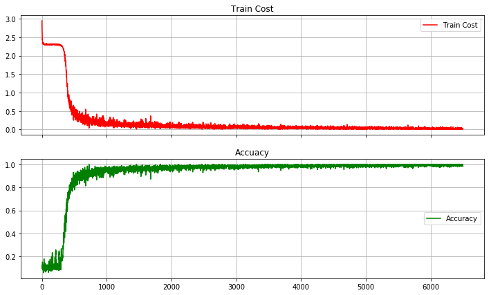
print 'Training Finish !'epoch : 10,cost:2.29978,accu:0.11328 epoch : 20,cost:0.46377,accu:0.87500 epoch : 30,cost:0.10498,accu:0.96875 epoch : 40,cost:0.26420,accu:0.92188 epoch : 50,cost:0.14124,accu:0.96484 epoch : 60,cost:0.06719,accu:0.97656 epoch : 70,cost:0.05444,accu:0.97266 epoch : 80,cost:0.06638,accu:0.98047 epoch : 90,cost:0.04561,accu:0.99219 epoch : 100,cost:0.02032,accu:0.99609 epoch : 110,cost:0.03399,accu:0.98828 epoch : 120,cost:0.04614,accu:0.98438 epoch : 130,cost:0.02753,accu:0.99219 Training Finish !
Training loss and accuracy
fig, (ax1, ax2) = plt.subplots(2, sharex=True, figsize=(12,7))
ax1.plot(Cost,label='Train Cost',c='red')
ax1.set_title('Train Cost')
ax1.grid(True)
ax1.legend(loc=0)
ax2.set_title('Accuacy')
ax2.plot(Accu,label='Accuracy',c='green')
ax2.grid(True)
plt.legend(loc=5)
plt.show()
Test accuracy
test_images = mnist.test.images
test_labels = mnist.test.labels
test_accuracy = sess.run(accuracy, feed_dict={images:test_images, labels:test_labels, keep_prob:1.0})
print 'Test Accuracy is: %.5f'%(test_accuracy)
Test Accuracy is: 0.98800
The test results are less than 99.2%. There may be several reasons for this:
1. No data enhancement processing is used
2. The number of convolution cores has also been reduced a lot.
3. The parameter t of the model can also be increased appropriately, because batchsize=256, 50 times are selected randomly. The training data of each round can not cover the training data completely, and the training data size is 55000.
3. In order to speed up the training, the network was streamlined, three LRNs were removed and two pools were pooled.
4. Maybe MNIST data is too small to fully reflect AlexNet
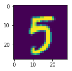
training sample
# A sample is selected from the training data and converted into an array of 28x28.
fig2,ax2 = plt.subplots(figsize=(2,2))
ax2.imshow(np.reshape(mnist.train.images[28], (28, 28)))
plt.show()
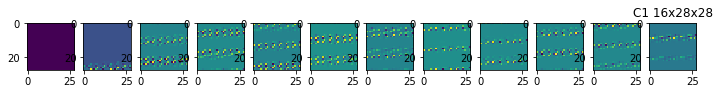
Convolution 1
# Characteristic diagram of convolution output of the first layer (no, activation, LRN, pooling)
input_image = mnist.train.images[28:29]
C1 = sess.run(c1, feed_dict={images:input_image})              # [1, 28, 28 ,12]
C1_reshape = sess.run(tf.reshape(C1, [12, 1, 28, 28]))
fig3,ax3 = plt.subplots(nrows=1, ncols=12, figsize = (12,2))
for i in range(12):
    ax3[i].imshow(C1_reshape[i][0])                            # tensor slices [batch, channels, row, column]
plt.title('C1 16x28x28')
plt.show()
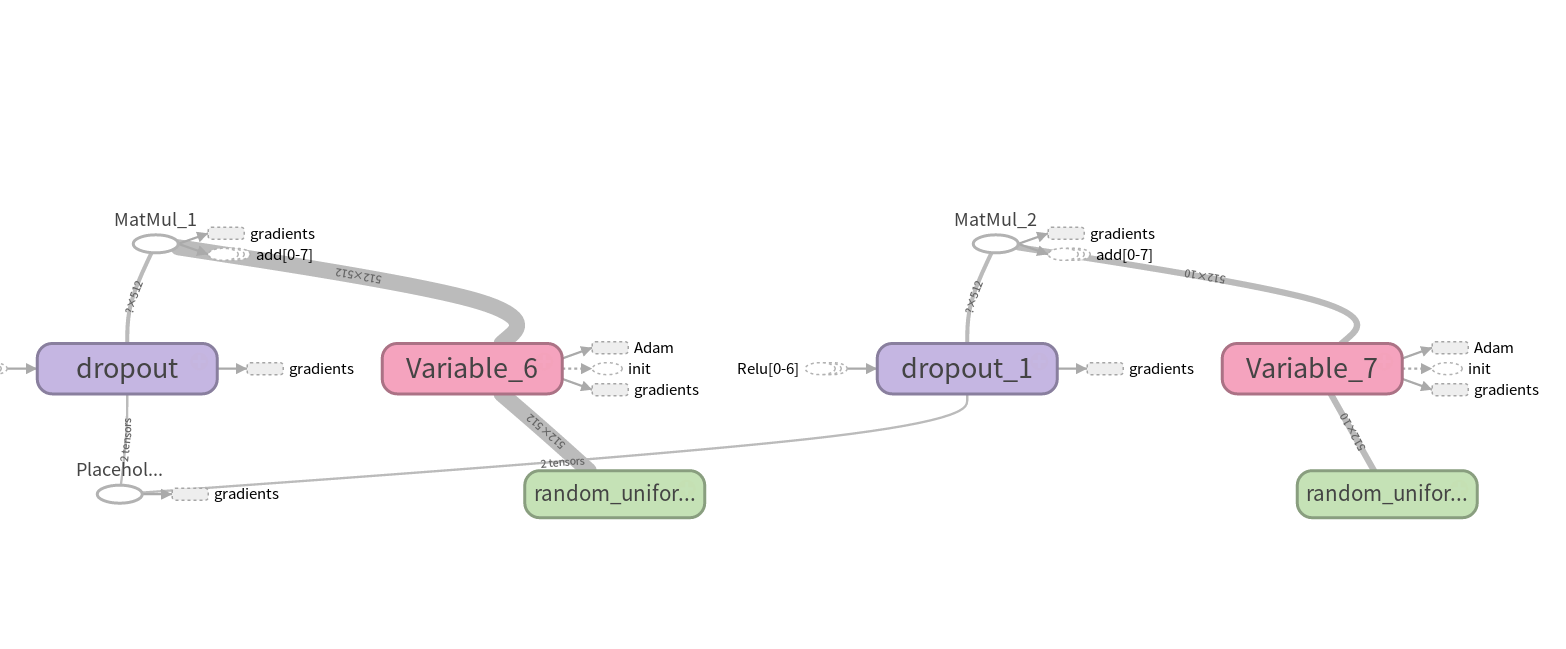
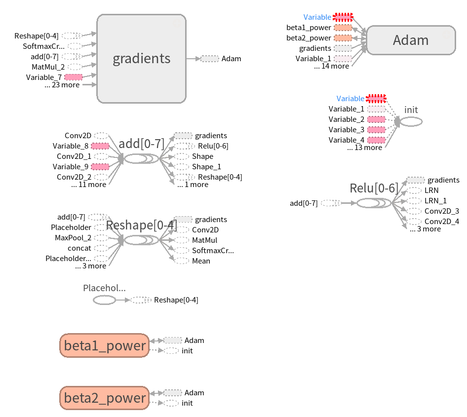
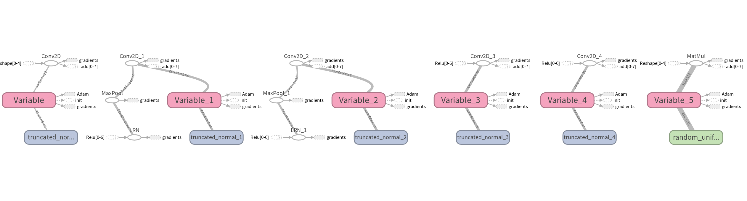
TensorBoard Visual Network
Five convolutional layers 
Full connection