First, the first question: what is tensorflow? It is an open source software library for solving numerical calculation based on data flow graph. Now it is mainly used for in-depth learning. In my understanding, tensorflow can complete the construction of neural network and carry out a series of data calculation (including linear change, activation function, etc.).
Second, what is tensor? By searching the notes of the major gods, we can understand this: tensor is also called tensor. It is a bucket of data in the whole framework. It represents all forms of data with N-dimensional vectors.
To sum up from my learning video at station b, I think the application of tensorflow in deep learning provides many encapsulated methods. Developers can directly use these methods to build deep networks, optimize and adjust parameters, which greatly simplifies the development process. The following is a summary of the knowledge learned:
1.1 basic build statements
import tensorflow as tf
import pandas as pd
import numpy as np

path=r'C:\Users\Poof poop poop poop poop poop poop poop poop pi\Desktop\machine learning-data\ex1data1.txt'
data=pd.read_csv(path,names=['educ','income'])#Read data
x=data.educ
y=data.income
model=tf.keras.Sequential()#Constructing neural network model
model.add(tf.keras.layers.Dense(1,input_shape=(1,)))#Build a hidden layer: ax+b is calculated
model.summary()
model.compile(optimizer='adam',loss='mse')#Optimize the algorithm to obtain the minimum a and b. the gradient descent is here. Optimizer is the optimizer
model.fit(x,y,epochs=500)#Training model, epochs is the number of training
print(model.predict(x))#Use model prediction
tf.keras.Sequential() is to build a sequential model, which is a sequential model. It is applicable to relatively simple networks with only one input and one output (what should I do when there are multiple outputs or inputs? Write later)
model.add() is used to add layers, and tf.keras.layers.Dense () is used to build a full connection layer.
Pay attention to the optimization function: adam optimization algorithm is a commonly used algorithm, which has good robustness to super parameters. It is a first-order optimization algorithm that can replace the traditional random gradient descent process, and can give the updated neural network weight of training data iteration.
When the learning rate needs to be set manually: model.compile(optimizer=tf.keras.opyimizers.Adam(learning_rate=0.01))
model=tf.keras.Sequential([tf.keras.layers.Dense(10,input_shape(3,),activation=relu)
                            tf.keras.layers.Dense(1)])
This model is built in two layers. When the activation function uses relu (well-known activation function and sigmoid), the output is 1 number.
1.2 loss function
model.compile(optimizer='adam',loss='binary_crossentropy',metrics=['acc'])
The loss function used in this model is the loss function in logistic regression, metrics It represents accuracy
Look carefully, the loss function here is binary_ Crossintropy, the formula is:

In the previous example, the loss function uses loss, and the formula is:

There are also two loss functions, spark_ categorical_crossentropy,categorical_ crossentropy.
1.3 multi classification problem
The multi classification problem is literal. Many classifications, different from the two classifications, can be represented by 0 and 1. It needs to output multiple probabilities. The category with the largest probability is its prediction category. This course introduces a collection of clothing images: fashion minist, 70000 images in total, call the data set:
(train_image,train_lable),(test_amage,test_lable)=tf.keras.datasets.fashion_mnist.load_data()

model.add(tf.keras.layers.Flatten(input_shape=(28,28)))
#The Flattern function smoothes the two-dimensional input image into a one-dimensional vector. The two-bit vector cannot be directly used in the Dense layer

model.add(tf.keras.layers.Dense(10,activation='softmax'))
Note that when the probability of multi classification needs to be output, softmax needs to be used as the activation function in the output layer instead of relu or sigmoid.
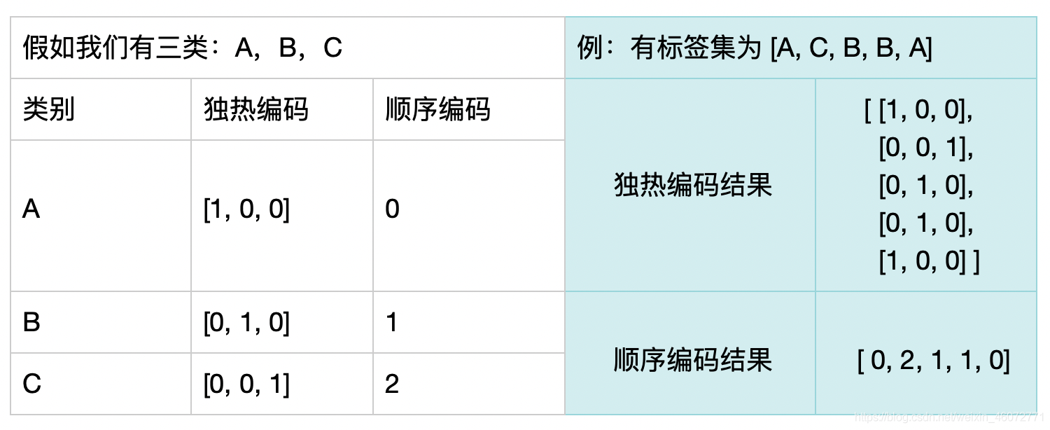
1.4 loss function of sequential coding and one hot coding
First, use a diagram to distinguish between sequential coding and heat only coding:

When the data is sequentially encoded, the loss function is sparse_categorical_crossentropy
When the data is uniquely hot coded, the loss function is categorical_crossentropy
Sequential coding and single heat coding can be converted to each other:
test_lable_onehot=tf.keras.utils.to_categorical(test_lable)
1.5 network capacity
Network capacity: it is directly proportional to the trainable parameters in the network. The more neural units and layers in the network, the stronger the fitting ability. However, if the training speed and difficulty are too large, the easier it is to produce over fitting. Methods to suppress over fitting: regularization, dropout, etc. Dropout is to artificially lose some neurons, making the network more streamlined:
model.add(tf.keras.layers.Dropout(0.5)) With a probability of 0.5, half of the neurons go out
Improve network fitting ability:
1. Add layer (this is more effective)
2. Increase the number of hidden neurons
1.6 function api
Compared with the set sequential model, it is more flexible to use the function api to build a neural network. Sequential has only one input and one output. Compared with restrictions, the function api can decide the input and output, multi input and multi output. I think it can be understood as follows: sequential is a model house, you can build a house according to this model house, and the function api is A piece of white paper, you only have basic building materials and can build your own house. An example:
input=keras.Input(shape=(28,28)) establish input

x=keras.layers.Flatten()(input)

x=keras.layers.Dense(32,activation='relu')(x)

x=keras,layers.Dropout(0.5)()

x=keras.layers.Dense(64,activation='relu')(x)

output=keras.layers.Dense(10,activation='softmax')(x) establish output

model=keras.Model(inputs=input,outputs=output) use input Follow output Model building

model.summary()
Learning video: Tensorflow 2.0 introduction and practice the most easy to understand course in 2019