1. Tensor data type

TensorFlow is not so mysterious. In order to adapt to automatic derivation and GPU operation, it came into being. In order to fit with the core data type ndarray of numpy, the core data type is Tensor, which means Tensor in Chinese (generally, it is mathematically divided into scalar, one-dimensional vector and two-dimensional matrix. The two-dimensional above is called Tensor. Of course, Tensor type is used in TF2). Variable is a package of Tensor, which enables Tensor to have the ability of automatic derivation (that is, it can be optimized. This type is specially set for neural network parameters).

Tensor value types are:

• int, float, double
• bool
• string

1. Define tensor

# Define constants, ordinary tensor s
tf.constant(1)
tf.constant(1.)
tf.constant([True,False])
tf.constant('hello nick')

1. attribute

with tf.device('cpu'):
    a = tf.constant([1])
with tf.device('gpu'):
     b = tf.constant([1])
# Device properties
print(a.device)
# cpu to GPU
print(a.gpu())
# Get numpy data type
print(a.numpy())
# Get the properties of a
print(a.shape)
# Get dimension of a
print(a.ndim)
# Get dimension
print(tf.rank(a))

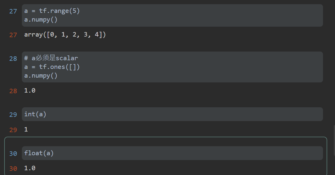
1. Data type judgment

# Judge whether it is tensor
print(isinstance(a, tf.Tensor))
print(tf.is_tensor(a))
print(a.dtype)
print(b.dtype)

1. Data type conversion

import numpy as np
a = np.arange(5)
print(a)
# numpy to tensor
aa = tf.convert_to_tensor(a, dtype=tf.int32)
print(aa)
# Data type conversion between tensor s
aaa = tf.cast(aa, dtype=tf.float32)
print(aaa)
# int to bool
b = tf.constant([0, 1])
print(b)
bb = tf.cast(b, dtype=tf.bool)
print(bb)

• Variable
  Create and use Tensor, except for trainable and other attributes.

a = tf.convert_to_tensor(np.arange(10))
b = tf.Variable(a)
print(b)
print(tf.is_tensor(b))
print(isinstance(b, tf.Tensor))
#%%
# tf.Variable
a = tf.range(5)
# After the tensor is changed to Variable, it has the characteristic of derivation, that is, it automatically records the gradient related information of a
b = tf.Variable(a)
print(b.name)
#%%
b = tf.Variable(a, name='input_data')
print(b.name) # input_data
print(b.trainable) # True
#%%
print(isinstance(b, tf.Tensor)) # False
print(isinstance(b, tf.Variable)) # True
print(tf.is_tensor(b)) # True recommended

1. tensor to numpy
   

2. Create Tensor

1)from numpy or list
Tensor flow tensors can be generated directly from numpy matrices or Python list s that conform to matrix rules.

#%%
# numpy
print(tf.convert_to_tensor(np.ones([3,3])))
#%%
print(tf.convert_to_tensor(np.zeros([2,3])))
#%%
# list
print(tf.convert_to_tensor([1,2]))
print(tf.convert_to_tensor([[2],[3.]]))

1. Method creation
   tf.zeros: accept shape as the parameter and create a tensor of all 0.
   tf.zeros_like: accept the parameter as tensor, and create a tensor based on all 0 of the shape of the tensor.
   tf.ones: similar to TF zeros
   tf.ones_like: similar to TF zeros_ like
   tf.random.normal: accept the parameters shape, mean, stddev, create the tensor of the specified shape, and sample the data from the normal distribution of the specified mean and standard deviation.
   tf.random.truncated_normal: accept the same parameters as above, create the tensor of the specified shape, and sample the data after truncating from the normal distribution of the specified mean and standard deviation.
   tf.random.uniform: accept shape, minval and maxval as parameters, create a tensor of the specified shape, and generate data from the uniform distribution between the specified minimum value and the maximum value.
   tf.range: accept the parameter limit and create a one-dimensional tensor from start to limit.
   tf.constant: similar to TF convert_ to_ tensor.

# zeros
print(tf.zeros([]))
print(tf.zeros([1]))
print(tf.zeros([2,2,2]))
#%%
a = tf.zeros([2,3,4])
print(tf.zeros_like(a))
#%%
print(tf.random.uniform([2,2],minval=0, maxval=1))
print(tf.random.uniform([2,2],minval=0, maxval=1, dtype=float))
#%%
print(tf.range(10))
print(tf.range(10, 100, delta=3, dtype=tf.int32))
# ones
print(tf.ones(1))
print(tf.ones([]))
print(tf.ones([2]))
print(tf.ones([2, 3]))
# fill
print(tf.fill([2, 2], 0))
print(tf.fill([2, 2], 0))
# random
# Normal distribution, mean 1, variance 1
tf.random.normal([2, 2], mean=1, stddev=1)
# Truncated normal distribution,
tf.random.truncated_normal([2, 2], mean=0, stddev=1)
# uniform distribution
tf.random.uniform([2, 2], minval=0, maxval=1)
# After disrupting idx, the indexes of a and b remain unchanged
idx = tf.range(10)
print(idx)
idx = tf.random.shuffle(idx)
print(idx)
a = tf.random.normal([10, 784])
print(a)
b = tf.random.uniform([10], maxval=10, dtype=tf.int32)
print(b)
#%%
a = tf.gather(a, idx)
b = tf.gather(b, idx)
b
#%%
# constant
print(tf.constant(1))
print(tf.constant([1]))
print(tf.constant(tf.constant([1, 2.])))
print(tf.constant([[1, 2], [3., 2]]))

1. loss calculation

• loss without bias

# Unbiased loss
out = tf.random.uniform([4, 10])
print(out)

• one-hot

# one-hot
y = tf.range(4)
y = tf.one_hot(y, depth=10)
print(y)

• mse

# mse
loss = tf.keras.losses.mse(y, out)
print(loss)

• mean loss

loss = tf.reduce_mean(loss)
print(loss)

3. Tensor index and slice

1) C language style: index through multi-layer subscripts.
2) numpy style: through multi-level subscript index, it is written in a square bracket, separated by commas.
3) Python style: array[start:end:step, start:end:step,...] By default, start and end are from start to end by default. At the same time, by default, the first dimension is taken, several colons are taken from the beginning, and all the remaining dimensions are taken. Similarly, the above ellipsis indicates that the following dimensions are taken, which is equivalent to the meaning of not writing (however, when the ellipsis appears in the middle, it cannot be left blank).
4)selective index:
- tf.gather(a, axis, indices): axis represents the specified collection dimension, and indices represents the serial numbers collected on the dimension.
- tf.gather_nd(a, indices): indices can be multidimensional and indexed according to the specified dimension.
- tf.boolean_mask(a, mask, axis): index the True correspondence according to the Boolean mask (multi-layer dimensions are supported).

#%%
# Index by multiple subscripts.
array = tf.random.uniform([3,4,5,6],maxval=100, dtype=tf.int32)
print(array[0][0])
print(array[0][0][1])
print(array[0][0][1][-1]) # A negative subscript indicates a reverse search

#%%
# Use Python style
array = tf.random.uniform([2,3])
print(array[:,:].shape)
print(array[:,0].shape)
print(array[:,::2].shape)
# Reverse order: - 1
print(array[:-1,:].shape)

print(array[:].shape)
# ellipsis...
print(array[:,...].shape)
print(array[::,::].shape)


#%%
# selective index
a = tf.random.uniform([4,35,3])
print(tf.gather(a,axis=0, indices=[0,1,3]).shape) # gather
print(tf.gather_nd(a, [[0,1,2],[1,2,0]]).shape) # gather_nd
print(tf.boolean_mask(a, mask=[True,True, False,False],axis=0).shape) # boolean_mask

4. Tensor dimension transformation

• tf.reshape(a, shape): adjusting Tensor to a new legal shape will not change the data, but only the way of understanding the data. (specifying the dimension in reshape as - 1 means automatic derivation, similar to numpy)
• tf. Transfer (a, perm): transpose the original Tensor according to the dimension order specified by perm
• tf.expand_dims(a, axis): adds a new empty dimension before (axis is positive) or after (axis is negative) the specified dimension.
• tf.squeeze(a, axis): deletes the specified dimension that can be removed (the dimension value is 1).

#%%
# Adjusting Tensor to a new legal shape will not change the data
a = tf.random.uniform([16, 28, 28, 3])
print(a.shape, " ", a.ndim)
print(tf.reshape(a, [16, 28*28, 3]).shape)
print(tf.reshape(a, [16, -1, 3]).shape)
print(tf.reshape(a, [16,28*28*3]).shape)
print(tf.reshape(a, [16,-1]).shape)
#%%
array = tf.random.normal([4, 28, 28, 3])
b = tf.reshape(tf.reshape(array, [4, -1]), [4, 28, 28, 3]).shape
b
#%%
tf.reshape(tf.reshape(array, [4, -1]), [4, 14, 56, 3]).shape

#%%
tf.reshape(tf.reshape(array, [4, -1]), [4, 1, 784, 3]).shape


#%%
# Transpose the original Tensor according to the dimension order specified by perm
a = tf.random.uniform([16, 28, 28, 3])
print(tf.transpose(a, [0,3,1,2]).shape) # Transpose

#%%
# Add dimension
a = tf.random.normal([4,35,8])
print(tf.expand_dims(a, axis=0).shape)
print(tf.expand_dims(a, axis=3).shape)

#%%
# Extrusion dimension
a = tf.random.normal([1,28,28,1])
print(tf.squeeze(a,axis=0).shape)
print(tf.squeeze(a,axis=3).shape)
print(tf.squeeze(a,axis=-1).shape)

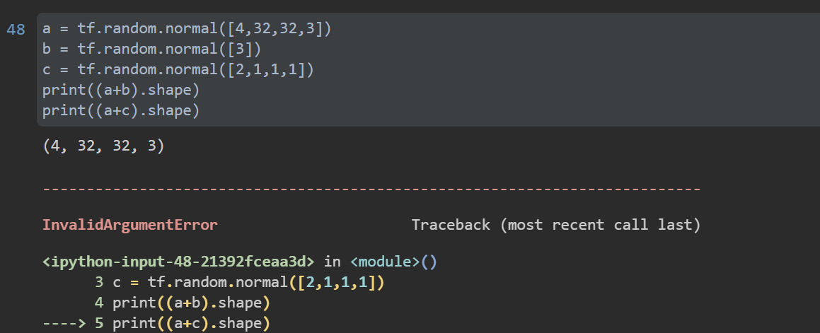
5. Broadcast

When tensors of different dimensions perform related operations, they need to unify the dimensions. Broadcast generally adds an empty dimension first, and then copies the original data along this dimension (in fact, it is not copied in storage). In TensorFlow, broadcast operation is performed automatically. Of course, TF can also be called broadcast_ To (a, target_shape).
Broadcast makes coding quite concise and saves memory space. However, when the expand step cannot be carried out, broadcast will fail and an error will be reported.

Broadcasting can be understood as dividing dimensions into large dimensions and small dimensions. Small dimensions are more specific and large dimensions are more abstract. That is, the small dimension is for an example, and then make the example common to the large dimension.


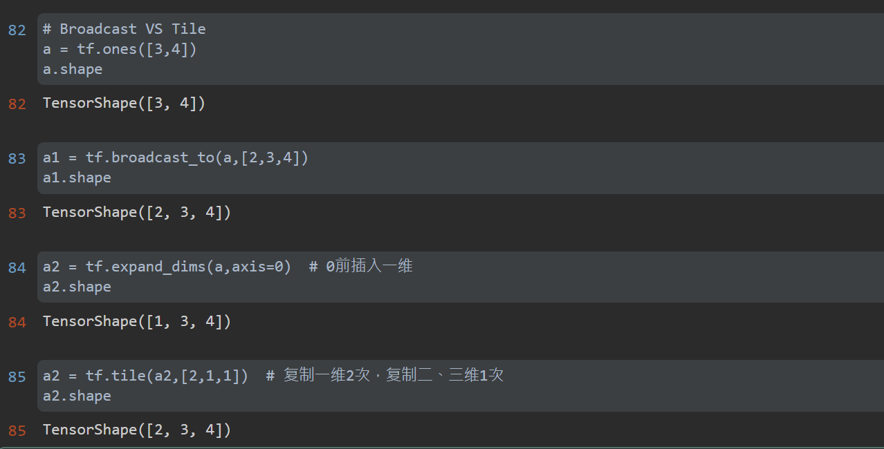
Broadcast VS Tile

6. Mathematical operation

1. Element operation: basic addition, subtraction, multiplication and division, that is, the elements at the corresponding position of the matrix perform these four mathematical operations.
2. Matrix operation: the operation between matrices conforms to the operation rules of matrices, mainly matrix multiplication.
3. Dimension operation: an operation on a dimension, reduce_mean,reduce_max and other methods.

# Element operation
a = tf.ones([2,2])
b = tf.fill([2,2],1.)
print(a+b)
print(a-b)
print(a*b)
print(a/b)
print(a//b)
print(a%b)
# tf.math.log, tf.exp
print(tf.math.log(a))
#%%
b = tf.fill([2, 2], 2.)
a = tf.ones([2, 2])
tf.exp(a)
#%%
tf.pow(b, 3)
#%%
tf.sqrt(b)
# Matrix operation
a = tf.random.normal([2,3])
b = tf.random.normal([3,4])
# @, matmul
print(a@b)
print(tf.matmul(a,b))
# Dimension operation
a = tf.random.normal([2,3,4])
print(tf.reduce_mean(a,axis=0))
print(tf.reduce_mean(a, axis=2))
# With broadcasting
#%%
a = tf.ones([4, 2, 3])  # 4 as batch
b = tf.fill([4, 3, 5], 2.)  # 4 as batch
#%%
a.shape
#%%
b.shape
#%%
bb = tf.broadcast_to(b, [4, 3, 5])
a@bb
#%%
# Y = X@W +b
x = tf.ones([4, 2])
W = tf.ones([2, 1])
b = tf.constant(0.1)  # Automatic broadcast is [4,1]
x@W + b
#%%
out = x@W + b
tf.nn.relu(out)

7. Handwritten numeral recognition process

1. MNIST handwritten numeral set 7000 * 10 pictures
2. 60k pictures are trained and 10k pictures are tested. Each picture is 2828. If it is a color picture, it is 2828 * 3
3. 0-255 represents the gray value of the picture, 0 represents pure white and 255 represents pure black
4. Flatten the matrix of 2828 to obtain a vector of 2828 = 784, and obtain [b,784] for B pictures; Then the encoding can be given for B pictures
5. The above ordinary codes are given as single heat codes, but the single heat codes are probability values, and the probability values are added to 1, which is similar to softmax regression
6. Apply the linear regression formula: X[b,784] W[784,10] b[10] to obtain [b,10]
7. The implementation of high-dimensional image is very complex, and a linear model can not be completed, so the nonlinear factor F can be added( X@W+b ), the activation function is used to make it nonlinear, and the relu function is derived
8. With the activation function, the model is still too simple. Use the factory
   • H1 =relu(X@W1+b1)
   • H2 = relu(h1@W2+b2)
   • Out = relu(h2@W3+b3)
     First, change [1784] to [1512] to [1256] to [1,10], get [1,10], and then code the result by using Euclidean distance or mse for error measurement, and [1784] outputs a [1,10] through a three-layer network

# -*- coding: utf-8 -*-#

# -------------------------------------------------------------------------------
# Name:         TranslationMNIST
# Description: read MNIST dataset and save it as a picture file
# Author:       PANG
# Date:         2021/7/24
# -------------------------------------------------------------------------------

import os

import tensorflow as tf
from tensorflow.keras import datasets

if __name__ == '__main__':
    os.environ['TF_CPP_MIN_LOG_LEVEL'] = '2'
    (x, y), _ = datasets.mnist.load_data()
    # transform Tensor
    # x: [0~255] ==> [0~1.]
    x = tf.convert_to_tensor(x, dtype=tf.float32) / 255.
    y = tf.convert_to_tensor(y, dtype=tf.int32)
    print(f'x.shape: {x.shape}, y.shape: {y.shape}, x.dtype: {x.dtype}, y.dtype: {y.dtype}')
    print(f'min_x: {tf.reduce_min(x)}, max_x: {tf.reduce_max(x)}')
    print(f'min_y: {tf.reduce_min(y)}, max_y: {tf.reduce_max(y)}')
    # batch of 128
    train_db = tf.data.Dataset.from_tensor_slices((x, y)).batch(128)
    train_iter = iter(train_db)
    sample = next(train_iter)
    print(f'batch: {sample[0].shape, sample[1].shape}')
    # [b,784] ==> [b,256] ==> [b,128] ==> [b,10]
    # [dim_in,dim_out],[dim_out]
    w1 = tf.Variable(tf.random.truncated_normal([784, 256], stddev=0.1))
    b1 = tf.Variable(tf.zeros([256]))
    w2 = tf.Variable(tf.random.truncated_normal([256, 128], stddev=0.1))
    b2 = tf.Variable(tf.zeros([128]))
    w3 = tf.Variable(tf.random.truncated_normal([128, 10], stddev=0.1))
    b3 = tf.Variable(tf.zeros([10]))
    # learning rate
    lr = 1e-3
    for epoch in range(10):  # iterate db for 10
        # train every train_db
        for step, (x, y) in enumerate(train_db):
            # x: [128,28,28]
            # y: [128]

            # [b,28,28] ==> [b,28*28]
            x = tf.reshape(x, [-1, 28 * 28])
            # only data types of tf.variable are logged
            with tf.GradientTape() as tape:
                # x: [b,28*28]
                # h1 = x@w1 + b1
                # [b,784]@[784,256]+[256] ==> [b,256] + [256] ==> [b,256] + [b,256]
                h1 = x @ w1 + tf.broadcast_to(b1, [x.shape[0], 256])
                h1 = tf.nn.relu(h1)
                # [b,256] ==> [b,128]
                # h2 = x@w2 + b2  # b2 can broadcast automatic
                h2 = h1 @ w2 + b2
                h2 = tf.nn.relu(h2)
                # [b,128] ==> [b,10]
                out = h2 @ w3 + b3
                # compute loss
                # out: [b,10]
                # y:[b] ==> [b,10]
                y_onehot = tf.one_hot(y, depth=10)
                # mse = mean(sum(y-out)^2)
                # [b,10]
                loss = tf.square(y_onehot - out)
                # mean:scalar
                loss = tf.reduce_mean(loss)

            # compute gradients
            grads = tape.gradient(loss, [w1, b1, w2, b2, w3, b3])
            # w1 = w1 - lr * w1_grad
            # w1 = w1 - lr * grads[0]  # not in situ update
            # in situ update
            w1.assign_sub(lr * grads[0])
            b1.assign_sub(lr * grads[1])
            w2.assign_sub(lr * grads[2])
            b2.assign_sub(lr * grads[3])
            w3.assign_sub(lr * grads[4])
            b3.assign_sub(lr * grads[5])

            if step % 100 == 0:
                print(f'epoch:{epoch}, step: {step}, loss:{float(loss)}')

8. TensorFlow realizes neural network

Here, the main functions of neural network are quickly introduced through TensorFlow amusement park. TensorFlow playground It is a simple neural network that can be trained through web browser and realize the visual training process.

• In machine learning, the combination of all numbers used to describe an entity is the feature vector of an entity.
• The feature vector is the input of the neural network.
• The neural network between input and output layers is called hidden layer. The more hidden layers, the deeper the neural network
• TensorFlow amusement park supports the number of nodes, learning rate, activation and regularization of each layer of neural network.
• Using neural network to solve classification problems can be divided into the following four steps:
  • 1. The feature vector of the entity in the problem is proposed as the input of the neural network.
  • 1. Define the structure of neural network and how to get the output from the input of neural network.
  • 1. The process of training neural network is to adjust the value of parameters in neural network through training data.
  • 1. The trained neural network is used to predict the unknown data.

reference material

1. TensorFlow: practical Google deep learning framework
2. https://www.cnblogs.com/nickchen121/p/10849484.html
3. https://zhouchen.blog.csdn.net/article/details/101790283