In the neural network optimization algorithm, the most commonly used method is the back propagation algorithm, and its work flow is as follows:
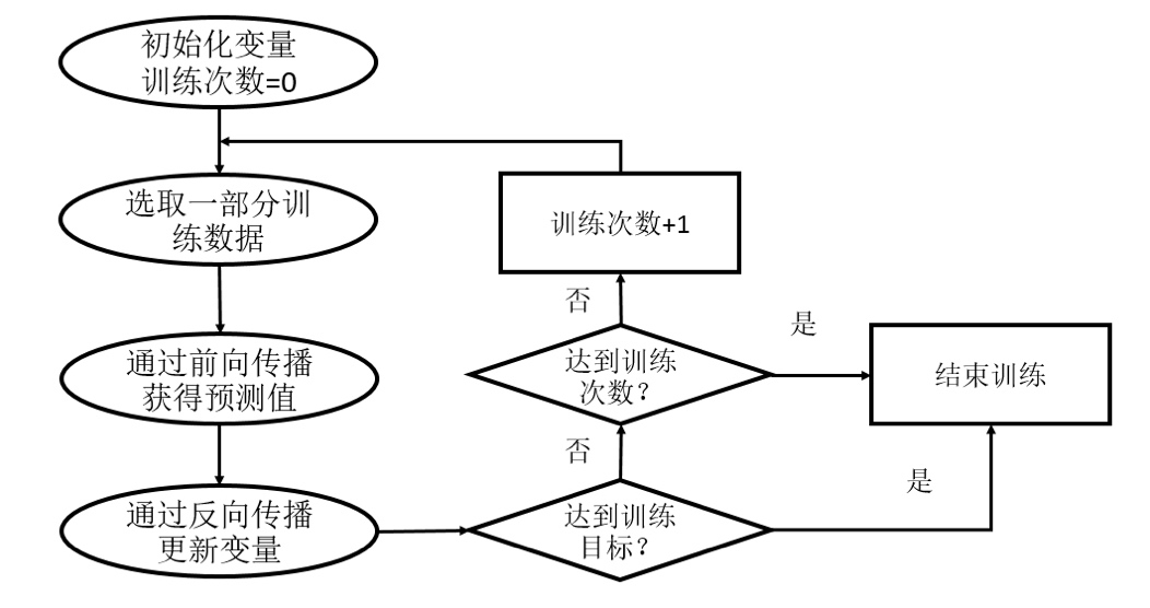
As shown in the figure, the back propagation algorithm implements an iterative process. At the beginning of each iteration, a part of training data is selected, which is called a batch. Then, the sample of this batch will get the prediction results of the neural network model through the forward propagation algorithm. Because the training data are marked with the correct answer, the gap between the predicted answer and the correct answer of the current neural network model can be calculated. Finally, based on this gap, the value of neural network parameters will be updated through the back-propagation algorithm, so that the prediction result of neural network on this batch is closer to the real answer.
Training of neural network model in TensorFlow v1
However, if the data selected in each iteration is represented by constants, the calculation diagram of TensorFlow will be large. Because TensorFlow will add a node in the calculation diagram every time a constant is generated. Generally speaking, the training process of a neural network will need to go through millions or even hundreds of millions of iterations, so the calculation diagram will be large and the utilization rate will be very low. The tensorplace provides a mechanism for inputting data. Placeholder is equivalent to defining a location, and the data in this location will be specified when the program runs. In this way, you only need to pass the data into TensorFlow calculation diagram through placeholder.
When the placeholder is defined, the data type at this location needs to be specified. Like tensors, the type of placeholder cannot be changed. The dimension information of the data in the placeholder can be derived from the provided data. The forward propagation algorithm implemented by placeholder (based on TensorFlow 2.5) is given below:
# -*- coding: utf-8 -*-#

# ----------------------------------------------
# Name:         NN02.py
# Description:
# Author:       PANG
# Date:         2022/2/5
# ----------------------------------------------
import tensorflow._api.v2.compat.v1 as tf  # Introduce TF1
tf.disable_v2_behavior() # Turn off v2 features

# Declare w1 and w2 variables, and fix the random seed through seed to ensure that the results of each run are the same
w1 = tf.Variable(tf.random_normal([2, 3], stddev=1, seed=1))
w2 = tf.Variable(tf.random_normal([3, 1], stddev=1, seed=1))

# Define the placeholder as the data storage place, and a given dimension can reduce the probability of error.
x = tf.placeholder(tf.float32, shape=(1, 2), name='input')
# Enter an N*m-dimensional array, where N is greater than 1.
xx = tf.placeholder(tf.float32, shape=(3, 2), name='input')
# Temporarily define the input eigenvector as a constant. X is a 1 * 2 matrix
# x = tf.constant([[0.7,0.9]])
a = tf.matmul(x, w1)
y = tf.matmul(a, w2)

aa = tf.matmul(xx, w1)
yy = tf.matmul(aa, w2)
sess = tf.Session()
init = tf.global_variables_initializer()
sess.run(init)

# print(sess.run(y))#An error will be reported. You need to provide a feed_dict to specify the value of x.
print(sess.run(y, feed_dict={x: [[0.7, 0.9]]}))
# When multidimensional array N*m is input, N*1 results are output
print(sess.run(yy, feed_dict={xx: [[0.7, 0.9], [0.1, 0.4], [0.5, 0.8]]}))
sess.close()
Note: feed_dict is a map, in which you need to give the value of each placeholder. If a required placeholder is not assigned a value, the program will report an error at run time.
After obtaining the forward propagation result of a batch, it is necessary to define a loss function to describe the gap between the current predicted value and the real answer. Then the back-propagation algorithm is used to adjust the value of neural network parameters, so that the gap can be narrowed.
# The loss function is defined to describe the gap between the predicted value and the real value
cross_entropy = -tf.reduce_mean(y_ * tf.log(tf.clip_by_value(y, 1e-10, 1.0)))
# Define learning rate
learning_rate = 0.001
# Back propagation algorithm is defined to optimize the parameters in neural network
train_step = tf.train.AdamOptimizer(learning_rate).minimize(cross_entropy)
TensorFlow v1 currently has seven optimizers, and there are three commonly used optimization methods:
- tf.train.GradientDescentOptimizer
- tf.train.AdamOptimizer
- tf.train.MomentumOptimizer
After defining the back propagation algorithm, run sess Run (train_step) can optimize the variables in the set to minimize the loss function of the current batch.
Complete neural network training program:
# -*- coding: utf-8 -*-#

# ----------------------------------------------
# Name:         NN02.py
# Description:
# Author:       PANG
# Date:         2022/2/5
# ----------------------------------------------
import numpy as np
import tensorflow._api.v2.compat.v1 as tf
# NumPy is a scientific computing toolkit that generates simulation data sets
from numpy.random import RandomState

tf.disable_v2_behavior()
# Define the size of training data batch
batch_size = 8

# Define the parameters of neural network
# Declare w1 and w2 variables. Here, the random seed is fixed through seed to ensure that the results of each run are the same
w1 = tf.Variable(tf.random_normal([2, 3], stddev=1, seed=1))
w2 = tf.Variable(tf.random_normal([3, 1], stddev=1, seed=1))

# Define the placeholder as the data storage point, and a given dimension can reduce the probability of error.
# Using None in one dimension of the shape makes it easy to use different batch sizes.
# It is necessary to divide the data into smaller batch es during training, but all the data can be used at one time during testing.
# When the data set is relatively small, this can facilitate testing, but when the data set is relatively large, putting a large amount of data into a batch will lead to data overflow.
x = tf.placeholder(tf.float32, shape=(None, 2), name='x-input')
# Enter an N*m-dimensional array, where N is greater than 1.
y_ = tf.placeholder(tf.float32, shape=(None, 1), name='y-input')

# Define the forward propagation process of neural network
a = tf.matmul(x, w1)
y = tf.matmul(a, w2)

# The loss function and back propagation algorithm are defined to describe the gap between the predicted value and the real value
y = tf.sigmoid(y)
cross_entropy = -tf.reduce_mean(
    y_ * tf.log(tf.clip_by_value(y, 1e-10, 1.0)) + (1 - y_) * tf.log(tf.clip_by_value(1 - y, 1e-10, 1.0)))
# Define learning rate
learning_rate = 0.001
# Back propagation algorithm is defined to optimize the parameters in neural network
train_step = tf.train.AdamOptimizer(learning_rate).minimize(cross_entropy)

# Generate an analog data set from random numbers
rdm = RandomState(1)
dataset_size = 128
X = rdm.rand(dataset_size, 2)

# The definition rule gives the label of the sample. In this example, X1 + x2 < 1 is considered as a positive sample,
# Others are negative samples. Here, use 0 to represent negative samples and 1 to represent positive samples
Y = [[int(x1 + x2 < 1) for (x1, x2) in X]]
Y = np.array(Y).reshape(-1, 1)
print(Y)
# Create a session to run the TensorFlow program
with tf.Session() as sess:
    init = tf.global_variables_initializer()
    sess.run(init)
    print(sess.run(w1))
    print(sess.run(w2))
    # Set training times
    Steps = 5000
    for i in range(Steps):
        # Each time batch is selected_ Two samples were trained
        start = (i * batch_size) % dataset_size
        # print(start)
        end = min(start + batch_size, dataset_size)
        # Through the selected samples, the neural network is trained and the parameters are updated
        sess.run(train_step, feed_dict={x: X[start:end], y_: Y[start:end]})

        if i % 1000 == 0:
            # The cross entropy of all data is calculated and output at regular intervals
            total_cross_entropy = sess.run(cross_entropy, feed_dict={x: X, y_: Y})
            print('loop:%d,Cross entropy:%g' % (i, total_cross_entropy))
    print(sess.run(w1))
    print(sess.run(w2))
Three steps of training neural network:
- Define the structure of neural network and the output result of forward propagation;
- Define the loss function and select the algorithm of back propagation optimization;
- Generate a session (tf.Session) and repeatedly run the back propagation optimization algorithm on the training data.
tf.Graph is the calculation model of TensorFlow. All TensorFlow programs will be represented in the form of calculation graph. Each node on the calculation graph is an operation, and the edge on the calculation graph represents the data transfer relationship between the operations. The edges on the calculation diagram also store the equipment information running each operation and the dependencies between the operations.
Tensor is the data model of TensorFlow. The input and output of all operations of TensorFlow are tensors. The tensor itself does not store any data, it is only a reference to the operation result.
Session is the operation model of TensorFlow. It manages the system resources owned by a TensorFlow program. All operations must be executed through the session.
Training of neural network in TensorFlow v2
Gradient descent method
gradient
∇
f
=
(
∂
f
∂
x
1
,
∂
f
∂
x
2
,
.
.
.
,
∂
f
∂
x
n
)
\nabla f=(\frac{\partial f}{\partial x_1},\frac{\partial f}{\partial x_2},...,\frac{\partial f}{\partial x_n} )
∂ f = (∂ x1 ∂ F, ∂ x2 ∂ F,..., ∂ xn ∂ f) refers to the derivative of the function with respect to the variable x. the direction of the gradient represents the direction in which the function value increases, and the modulus of the gradient represents the rate at which the function value increases. Then, as long as the value of the parameter is constantly updated to a certain size in the opposite direction of the gradient, the minimum value of the function (global minimum or local minimum) can be obtained
θ
t
+
1
=
θ
t
−
α
∇
f
(
θ
t
)
\theta _{t+1}=\theta _t-\alpha \nabla f(\theta _t)
θt+1=θt−α∇f(θt)
The above parameter updating process is called gradient descent method, but generally, when using gradient to update parameters, the gradient will be multiplied by a learning rate less than 1. This is because the modulus of gradient is often relatively large. Directly updating parameters with it will make the function value fluctuate continuously and it is difficult to converge to an equilibrium point.
However, for different functions, the gradient descent method may not be able to find the optimal solution. Many times, it can only converge to a local optimal solution and will not change, although this local optimal solution may be very close to the global optimal solution. Experiments show that the gradient descent method has a good performance for convex functions.
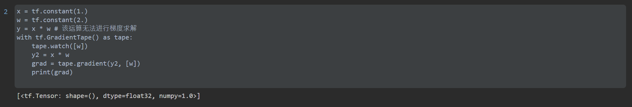
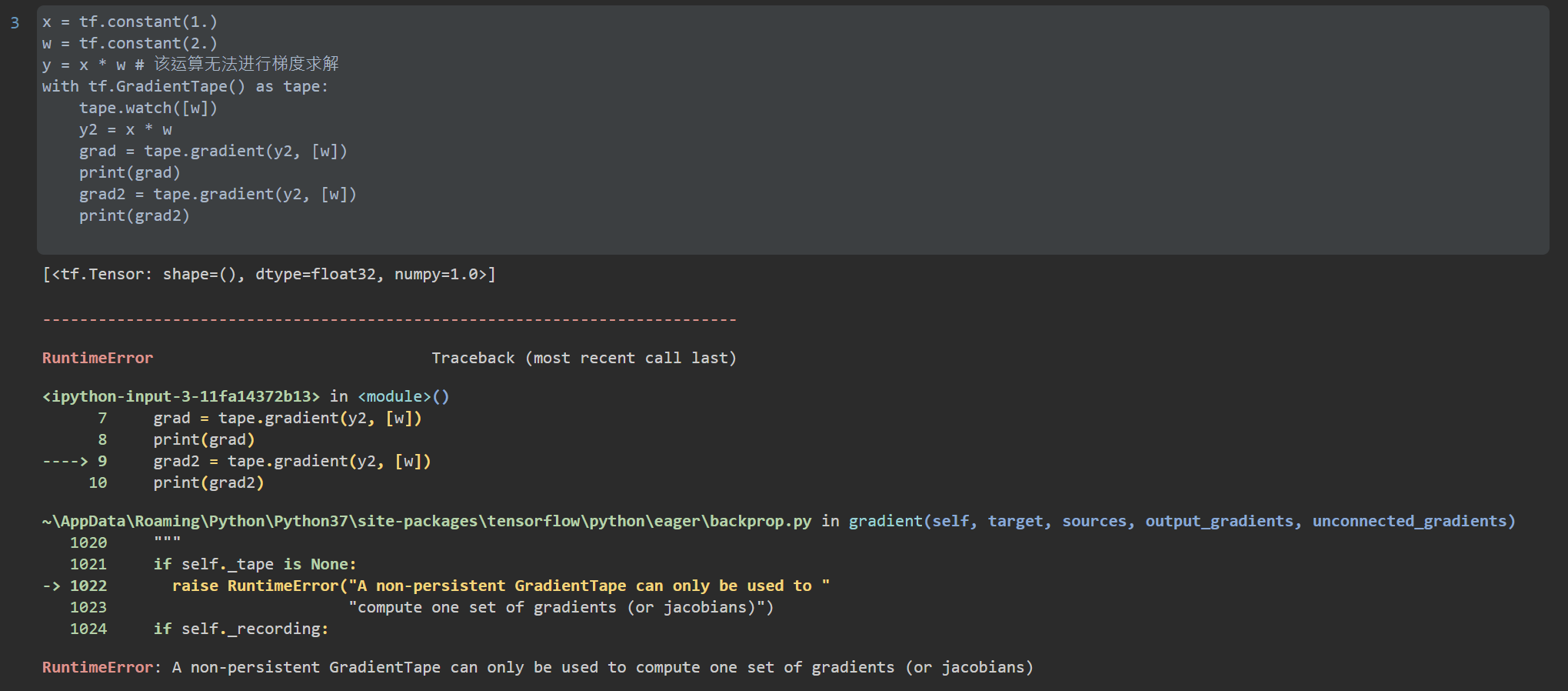
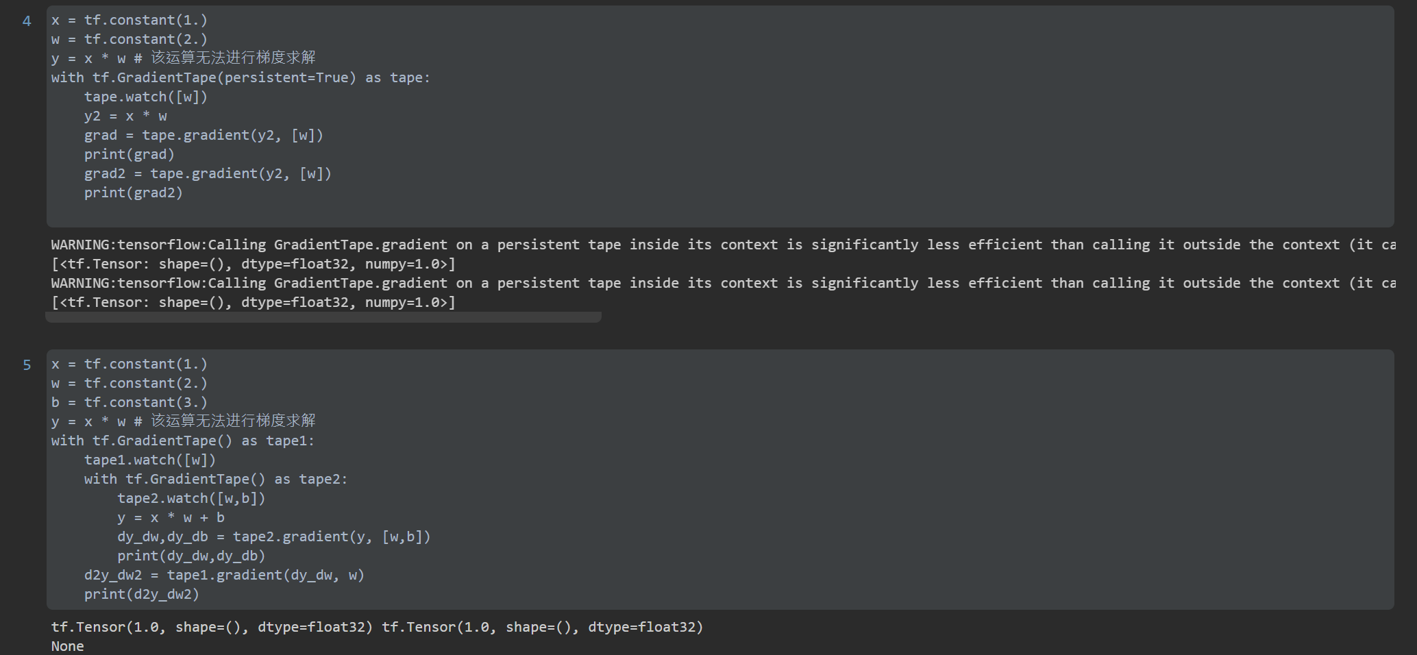
Deep learning frameworks such as TensorFlow and PyTorch support automatic gradient solution. In TensorFlow v2, TensorFlow will automatically solve the gradient of relevant operations as long as the code requiring gradient solution is wrapped in gradienttape. But through tape gradient(loss, [w1, w2,...]) It can only be called once. As a resource occupying a large amount of video memory, the gradient will be released after being obtained once. TF needs to be set to call multiple times GradientTape(persistent=True). TensorFlow v2 also supports multi-order derivation, which only needs to be wrapped multiple times. For example:
Back propagation
Back propagation algorithm (BP) is the core algorithm of training deep neural network. Its implementation is based on chain rule. The loss of the output layer is back propagated through the weight (the inverse operation of forward propagation) back to layer i (this is a process of repeated iterative return), and the gradient update parameters of layer i are calculated.
In tensorflow 2, the classical BP neural network layer is encapsulated, called the full connection layer, which automatically completes the operation of the hidden layer of BP neural network. The following is how to build BP neural network using Dense layer to train Fashion_MNIST data set to identify the code.
# -*- coding: utf-8 -*-#

# ----------------------------------------------
# Name:         NN03.py
# Description: back propagation algorithm example
# Author:       PANG
# Date:         2022/2/5
# ----------------------------------------------
import tensorflow as tf
from tensorflow.keras import datasets, layers, optimizers, Sequential

(x, y), (x_test, y_test) = datasets.fashion_mnist.load_data()
print(x.shape, y.shape)


def preprocess(x, y):
    x = tf.cast(x, dtype=tf.float32) / 255.
    y = tf.cast(y, dtype=tf.int32)
    return x, y


batch_size = 64
db = tf.data.Dataset.from_tensor_slices((x, y))
db = db.map(preprocess).shuffle(10000).batch(batch_size)
db_test = tf.data.Dataset.from_tensor_slices((x_test, y_test))
db_test = db_test.map(preprocess).shuffle(10000).batch(batch_size)

model = Sequential([
    layers.Dense(256, activation=tf.nn.relu),  # [b, 784] => [b, 256]
    layers.Dense(128, activation=tf.nn.relu),  # [b, 256] => [b, 128]
    layers.Dense(64, activation=tf.nn.relu),  # [b, 128] => [b, 64]
    layers.Dense(32, activation=tf.nn.relu),  # [b, 64] => [b, 32]
    layers.Dense(10),  # [b, 32] => [b, 10]
])
model.build(input_shape=([None, 28 * 28]))
optimizer = optimizers.Adam(lr=1e-3)


def main():
    # forward
    for epoch in range(30):
        for step, (x, y) in enumerate(db):
            x = tf.reshape(x, [-1, 28 * 28])
            with tf.GradientTape() as tape:
                logits = model(x)
                y_onthot = tf.one_hot(y, depth=10)

                loss_mse = tf.reduce_mean(tf.losses.MSE(y_onthot, logits))
                loss_ce = tf.reduce_mean(tf.losses.categorical_crossentropy(y_onthot, logits, from_logits=True))
            grads = tape.gradient(loss_ce, model.trainable_variables)
            # backward
            optimizer.apply_gradients(zip(grads, model.trainable_variables))

            if step % 100 == 0:
                print(epoch, step, "loss:", float(loss_mse), float(loss_ce))
        # test
        total_correct, total_num = 0, 0
        for x, y in db_test:
            x = tf.reshape(x, [-1, 28 * 28])
            logits = model(x)
            prob = tf.nn.softmax(logits, axis=1)
            pred = tf.cast(tf.argmax(prob, axis=1), dtype=tf.int32)
            correct = tf.reduce_sum(tf.cast(tf.equal(pred, y), dtype=tf.int32))
            total_correct += int(correct)
            total_num += int(x.shape[0])
        acc = total_correct / total_num
        print("acc", acc)


if __name__ == '__main__':
    main()
reference material
- TensorFlow: practical Google deep learning framework
- https://zhouchen.blog.csdn.net/article/details/102572264