0. Preface
Tensorflow is an open source machine learning framework based on Python. It is developed by Google and has rich applications in graphics classification, audio processing, recommendation system and natural language processing. It is one of the most popular machine learning frameworks at present. TensorFlow2.0 was released in October 2019 and has reached version 2.7.
Although many people are still using TF1 version, I think the future trend must be 2.0, and some old wheels will eventually be replaced by new wheels, so I started from 2.0. The code here mainly comes from the video course "artificial intelligence practice: tensorflow 2.0 notes" by Cao Jian, a teacher of Peking University. This article is a study note, which is mainly for your own query notes, not for commercial purposes. If there is infringement, please contact me.
1. Preparatory work
1.1 installation of Anaconda
Installation through anaconda is highly recommended here. Because Anaconda's base is really easy to use. It not only integrates the basic modules required by artificial intelligence, such as numpy, pandas, sklearn, matplotlib, but also facilitates environmental management and later upgrading. It is almost the only choice.
Official website address: https://www.anaconda.com/distribution/
Of course, there is no exception in installing such program software. If you can use domestic image, you can use domestic image.
Tsinghua mirror address: https://mirrors.tuna.tsinghua.edu.cn/anaconda/archive/
I chose anaconda3-5.3.1-windows-x86 here_ 64.exe version
Because it needs to be reinstalled on different machines frequently, just download it and save the source file. When you need to use it, double-click it directly to install it.
There was not much to say during the installation process, so I followed the prompts all the way. Note the python version. I chose Python 3 Version 8.5.
After installing anaconda, in fact, many basic modules of the environment required for artificial intelligence have been installed (of course, some are not suitable for TF2.0 and need to be upgraded), as well as Python. Next, install tensorflow2 0.
1.2,TensorFlow2.0 installation
Enter the prompt interface of Anaconda. If you want to create a new environment, you can use:
conda create environment name
To create an environment. If you want to switch environments, you can use
conda activate environment name} switch to the environment you want to use
Use the pip command to install TF2. Similarly, we can use the image if we can use the image:
Install tensorflow:
Specified version
pip3 install -i https://pypi.tuna.tsinghua.edu.cn/simple --upgrade tensorflow==1.12
Install the latest
pip3 install -i https://pypi.tuna.tsinghua.edu.cn/simple tensorflow
tips:
Error encountered while installing tensorflow: cannot uninstall 'wrap' It is a distutils installed project and thus we cannot accurately determine which files belong to it which would lead to only a partial uninstall.
Enter the following statement
pip install -U --ignore-installed wrapt enum34 simplejson netaddr
Install the wrapt first, and then install tensorflow
1.3 installation in other environments
Some of the libraries that come with my version of anaconda cannot be adapted to TF2 0, to upgrade, similarly, we try to upgrade with image.
Upgrade and install numpy
pip3 install --upgrade numpy
Upgrade and install pandas
pip3 install -i https://pypi.tuna.tsinghua.edu.cn/simple --upgrade pandas
Upgrade and install matplotlib
pip3 install -i https://pypi.tuna.tsinghua.edu.cn/simple --upgrade matplotlib
Finally, if I'm used to using jupyter, upgrade jupyter again. I'm used to using vscode.
1.4 environment variable configuration
There are two types of environment variables.
1. System environment variables
System environment variable, as the name suggests, is a system variable. That is to say, once the system environment variable is configured, any user who uses this operating system (an operating system can generally set multiple users) can directly find the corresponding program in the doc command window through this environment variable
2. User environment variables
User environment variable, as the name suggests, belongs to a user alone. Generally, if it is configured by that user, it belongs to that user. Only users who configure this environment variable can use it
Generally speaking, in this computer - properties - advanced system settings - Advanced - environment variables
You can find the following interface of environment variables
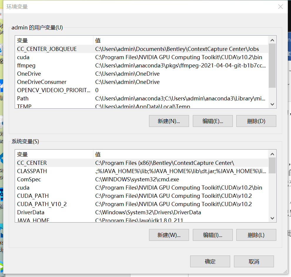
The above is the user variable and the following is the system variable. You can add both
Add the program address to be used to the list of environment variables.
For example, add my Anaconda variable address C:\Users\admin\anaconda3\Scripts.
After the above work is completed, test whether it is normal:
import tensorflow as tf
from tensorflow import keras
import matplotlib as mpl
import matplotlib.pyplot as plt
%matplotlib inline
import numpy as np
import sklearn
import pandas as pd
import os
import sys
import time


print(tf.__version__)
print(sys.version_info)
for module in mpl,np,pd,sklearn,tf,keras:
print(module.__name__,module.__version__)
After operation, the results are as follows:
2.7.0
sys.version_info(major=3, minor=7, micro=0, releaselevel='final', serial=0)
matplotlib 3.5.0
numpy 1.21.4
pandas 1.1.5
sklearn 0.19.2
tensorflow 2.7.0
keras.api._v2.keras 2.7.0
Note that my TensorFlow is version 2.7.0, followed by the versions of each module library. We will run our TensorFlow code in this environment.
2. Basic knowledge
2.1 tensor
Tensor in TensorFlow is tensor. In fact, it is a multidimensional array, and the dimension of tensor is expressed by order.
The tensor of order 0 is scalar, which represents a single number, such as s=5
The first-order tensor is a vector, which represents a one-dimensional array, such as v=[1,2,3]
The second-order tensor is a matrix, which represents a two-dimensional array, such as m=[[1,2,3],[4,5,6]]
N-order tensors are n-dimensional arrays
The data types of TensorFlow are
tf.int , tf.float: tf.int 32 tf.float32 tf.float64
tf.bool: tf.constant([True,False])
tf.string: tf.constant('Hello,world')
Method of creating tensor:
Tf. Constant (tensor content, dtype = data type (optional))
#Example 2-1: create a one-dimensional tensor
import tensorflow as tf
a=tf.constant([2,5],dtype=tf.int64)
print(a)

#Printed results:
tf.Tensor([2 5], shape=(2,), dtype=int64)
tf. convert_ to_ The tensor function can change data in numpy format into data in tensor format
#Example 2-2: using convert_to_tensor created by tensor function
import numpy as np
b=np.arange(0,5)
c=tf.convert_to_tensor(b,dtype=tf.int64)
print(b)
print(c)

#The printing results are as follows:
[0 1 2 3 4]
tf.Tensor([0 1 2 3 4], shape=(5,), dtype=int64)
tf. Zeros (dimension) creates tensors with all zeros
tf. The ones (dimension) creates tensors that are all 1
tf. Fill (dimension, specified value) creates a tensor with all specified values
#Example 2-3: create tensors with zeros, ones and fill functions
d=tf.zeros([3,4])
e=tf.ones([3,2])
f=tf.fill([3,3],8)
print(d)
print(e)
print(f)

Print results:
tf.Tensor(
[[0. 0. 0. 0.]
 [0. 0. 0. 0.]
 [0. 0. 0. 0.]], shape=(3, 4), dtype=float32)
tf.Tensor(
[[1. 1.]
 [1. 1.]
 [1. 1.]], shape=(3, 2), dtype=float32)
tf.Tensor(
[[8 8 8]
 [8 8 8]
 [8 8 8]], shape=(3, 3), dtype=int32)
tf. random. Normal (dimension, mean = mean, stddev = standard deviation)
Generate random numbers that conform to normal distribution. The default mean is 0 and the standard deviation is 1
Tf. random. truncated_ Normal (dimension, mean = mean, stddev = standard deviation)
Generating random numbers with truncated normal distribution
Tf. random. Uniform (dimension, minval = minimum, maxval = maximum)
Generates a uniformly distributed random number with a specified maximum and minimum value
#Example 2-4: generate different types of random number tensor s
g=tf.random.normal([3,2],mean=3,stddev=1)
h=tf.random.truncated_normal([2,4],mean=5)
i=tf.random.uniform([4,5],minval=8,maxval=20)
print(g)
print(h)
print(i)

#Print results
tf.Tensor(
[[2.711913  2.7192001]
 [2.9681098 3.2150037]
 [2.3997366 2.749307 ]], shape=(3, 2), dtype=float32)
tf.Tensor(
[[4.66647   5.542239  4.4181    4.7608485]
 [6.2916203 5.4339285 5.40028   6.618659 ]], shape=(2, 4), dtype=float32)
tf.Tensor(
[[ 9.444313  16.606283   8.992081   9.405373  18.322927 ]
 [18.356173   9.4511795 17.346773   8.193683  15.328684 ]
 [13.65999    8.159064   9.28767   11.537907  13.05283  ]
 [10.011724  10.25061   12.929413  11.793535  19.735085 ]], shape=(4, 5), dtype=float32)
2.2 common functions
2.2.1,tf.cast is used to force type conversion, that is, force tensor to convert to this data type
Usage: TF Cast (tensor name, dtype = data type)
2.2.2,tf.reduce_min is used to calculate the minimum value of the element on the tensor dimension
Usage: TF reduce_ Min (tensor name)
2.2.3,tf.reduce_max is used to calculate the maximum value of the element in the tensor dimension
Usage: TF reduce_ Max (tensor name)
2.2.4,tf.reduce_mean is used to calculate the average value of elements in the tensor dimension
Usage: TF reduce_ Mean (tensor name, axis = operation axis)
2.2.5,tf.reduce_sum is used to calculate the sum of elements in the tensor dimension
Usage: TF reduce_ Sum (tensor name, axis = operation axis)
#Example 2-5: some operations of tensor
j=tf.constant([[1,2.34,3.76],[5.98,7.09,9.13]],dtype=tf.float64)
print(j)
j2=tf.cast(j,tf.int32)
print(j2)

j3=tf.reduce_min(j)
print(j3)
j4=tf.reduce_max(j)
print(j4)
j5=tf.reduce_mean(j2,axis=1)
print(j5)
j6=tf.reduce_sum(j2,axis=0)
print(j6)

#Print results

tf.Tensor(
[[1.   2.34 3.76]
 [5.98 7.09 9.13]], shape=(2, 3), dtype=float64)
tf.Tensor(
[[1 2 3]
 [5 7 9]], shape=(2, 3), dtype=int32)
tf.Tensor(1.0, shape=(), dtype=float64)
tf.Tensor(9.13, shape=(), dtype=float64)
tf.Tensor([2 7], shape=(2,), dtype=int32)
tf.Tensor([ 6  9 12], shape=(3,), dtype=int32)
2.2.6 variable function
Mark the variable as "trainable", and the marked variable will record the gradient information in the back propagation. This function is often used to mark the parameters to be trained in neural network training.
Usage: TF Variable (initial value)
#Example 2-6
import tensorflow as tf

w = tf.Variable(tf.constant(5, dtype=tf.float32))

epoch = 40
LR_BASE = 0.2  # Initial learning rate
LR_DECAY = 0.99  # Learning rate decay rate
LR_STEP = 1  # How many rounds of batch are fed_ After size, update the learning rate once

for epoch in range(epoch):  # For epoch defines the top-level cycle, which means that the data set is cycled for epoch times. In this example, the data set has only one w. during initialization, constant is assigned as 5, and the cycle is iterated for 100 times.
    lr = LR_BASE * LR_DECAY ** (epoch / LR_STEP)
    with tf.GradientTape() as tape:  # The calculation process of gradient from with structure to grads frame.
        loss = tf.square(w + 1)
    grads = tape.gradient(loss, w)  # The. gradient function tells who takes the derivative from whom

    w.assign_sub(lr * grads)  # .assign_sub makes self subtraction of variables, i.e. w -= lr*grads, i.e. w = w - lr*grads
    print("After %s epoch,w is %f,loss is %f,lr is %f" % (epoch, w.numpy(), loss, lr))


#Print results

After 0 epoch,w is 2.600000,loss is 36.000000,lr is 0.200000
After 1 epoch,w is 1.174400,loss is 12.959999,lr is 0.198000
After 2 epoch,w is 0.321948,loss is 4.728015,lr is 0.196020
After 3 epoch,w is -0.191126,loss is 1.747547,lr is 0.194060
After 4 epoch,w is -0.501926,loss is 0.654277,lr is 0.192119
After 5 epoch,w is -0.691392,loss is 0.248077,lr is 0.190198
After 6 epoch,w is -0.807611,loss is 0.095239,lr is 0.188296
After 7 epoch,w is -0.879339,loss is 0.037014,lr is 0.186413
After 8 epoch,w is -0.923874,loss is 0.014559,lr is 0.184549
After 9 epoch,w is -0.951691,loss is 0.005795,lr is 0.182703
After 10 epoch,w is -0.969167,loss is 0.002334,lr is 0.180876
After 11 epoch,w is -0.980209,loss is 0.000951,lr is 0.179068
After 12 epoch,w is -0.987226,loss is 0.000392,lr is 0.177277
After 13 epoch,w is -0.991710,loss is 0.000163,lr is 0.175504
After 14 epoch,w is -0.994591,loss is 0.000069,lr is 0.173749
After 15 epoch,w is -0.996452,loss is 0.000029,lr is 0.172012
After 16 epoch,w is -0.997660,loss is 0.000013,lr is 0.170292
After 17 epoch,w is -0.998449,loss is 0.000005,lr is 0.168589
After 18 epoch,w is -0.998967,loss is 0.000002,lr is 0.166903
After 19 epoch,w is -0.999308,loss is 0.000001,lr is 0.165234
After 20 epoch,w is -0.999535,loss is 0.000000,lr is 0.163581
After 21 epoch,w is -0.999685,loss is 0.000000,lr is 0.161946
After 22 epoch,w is -0.999786,loss is 0.000000,lr is 0.160326
After 23 epoch,w is -0.999854,loss is 0.000000,lr is 0.158723
After 24 epoch,w is -0.999900,loss is 0.000000,lr is 0.157136
After 25 epoch,w is -0.999931,loss is 0.000000,lr is 0.155564
After 26 epoch,w is -0.999952,loss is 0.000000,lr is 0.154009
After 27 epoch,w is -0.999967,loss is 0.000000,lr is 0.152469
After 28 epoch,w is -0.999977,loss is 0.000000,lr is 0.150944
After 29 epoch,w is -0.999984,loss is 0.000000,lr is 0.149434
After 30 epoch,w is -0.999989,loss is 0.000000,lr is 0.147940
After 31 epoch,w is -0.999992,loss is 0.000000,lr is 0.146461
After 32 epoch,w is -0.999994,loss is 0.000000,lr is 0.144996
After 33 epoch,w is -0.999996,loss is 0.000000,lr is 0.143546
After 34 epoch,w is -0.999997,loss is 0.000000,lr is 0.142111
After 35 epoch,w is -0.999998,loss is 0.000000,lr is 0.140690
After 36 epoch,w is -0.999999,loss is 0.000000,lr is 0.139283
After 37 epoch,w is -0.999999,loss is 0.000000,lr is 0.137890
After 38 epoch,w is -0.999999,loss is 0.000000,lr is 0.136511
After 39 epoch,w is -0.999999,loss is 0.000000,lr is 0.135146
2.2.7 four operations of corresponding elements
Four operations: addition: TF Add, subtract: TF Subtract, multiplication: TF Multiply, Division: TF divide
Square: TF square,
Power: TF pow
Prescription: TF sqrt
Matrix multiplication: TF matmul
#Example 2-7
import tensorflow as tf

k1 = tf.ones([1, 3])
k2 = tf.fill([1, 3], 3.)

print("k1:", k1)
print("k2:", k2)
print("k1+k2:", tf.add(k1, k2))
print("k1-k2:", tf.subtract(k1, k2))
print("k1*k2:", tf.multiply(k1, k2))
print("k2/k1:", tf.divide(k2, k1))

k3 = tf.fill([1, 2], 3.)
print("k3:", k3)
print("k3 The third power of:", tf.pow(k3, 3))
print("k3 Square of:", tf.square(k3))
print("k3 Formula of:", tf.sqrt(k3))

k4 = tf.ones([3, 2])
k5 = tf.fill([2, 3], 3.)
print("k4:", k4)
print("k5:", k5)
print("k4*k5:", tf.matmul(k4, k5))


#Print results:
k1: tf.Tensor([[1. 1. 1.]], shape=(1, 3), dtype=float32)
k2: tf.Tensor([[3. 3. 3.]], shape=(1, 3), dtype=float32)
k1+k2: tf.Tensor([[4. 4. 4.]], shape=(1, 3), dtype=float32)
k1-k2: tf.Tensor([[-2. -2. -2.]], shape=(1, 3), dtype=float32)
k1*k2: tf.Tensor([[3. 3. 3.]], shape=(1, 3), dtype=float32)
k2/k1: tf.Tensor([[3. 3. 3.]], shape=(1, 3), dtype=float32)
k3: tf.Tensor([[3. 3.]], shape=(1, 2), dtype=float32)
k3 The third power of: tf.Tensor([[27. 27.]], shape=(1, 2), dtype=float32)
k3 Square of: tf.Tensor([[9. 9.]], shape=(1, 2), dtype=float32)
k3 Formula of: tf.Tensor([[1.7320508 1.7320508]], shape=(1, 2), dtype=float32)
k4: tf.Tensor(
[[1. 1.]
 [1. 1.]
 [1. 1.]], shape=(3, 2), dtype=float32)
k5: tf.Tensor(
[[3. 3. 3.]
 [3. 3. 3.]], shape=(2, 3), dtype=float32)
k4*k5: tf.Tensor(
[[6. 6. 6.]
 [6. 6. 6.]
 [6. 6. 6.]], shape=(3, 3), dtype=float32)
2.2.8,tf.data.Dataset.from_tensor_slices is used to segment the first dimension of the incoming tensor, generate input feature tag pairs, and construct data sets
#Example 2-8
data=tf.data.Dataset.from_tensor_slices((Input features, labels))

features=tf.constant([15, 28, 34, 19])
labels=tf.constant([0,1,1,0])
dataset=tf.data.Dataset.from_tensor_slices((features,labels))
print(dataset)
for element in dataset:
    print(element)


#Print results

(<tf.Tensor: shape=(), dtype=int32, numpy=15>, <tf.Tensor: shape=(), dtype=int32, numpy=0>)
(<tf.Tensor: shape=(), dtype=int32, numpy=28>, <tf.Tensor: shape=(), dtype=int32, numpy=1>)
(<tf.Tensor: shape=(), dtype=int32, numpy=34>, <tf.Tensor: shape=(), dtype=int32, numpy=1>)
(<tf.Tensor: shape=(), dtype=int32, numpy=19>, <tf.Tensor: shape=(), dtype=int32, numpy=0>)
2.2.9,tf.GradientTape , find the gradient of the tensor
Usage:
with tf.GradientTape() as tape:
Calculation process
Grad=tape. Gradient (function, derivative to whom)
#Example 2-9:

With tf.gradientTape() as tape:

W=tf.Variable(tf.constant(3.0))

Loss=tf.pow(w,2)

Grad=tape.gradient(loss,w)

Print(grad)


#Print results:

tf.Tensor(6.0, shape=(), dtype=float32)
2.2.10 enumerate is a built-in function of python. It can traverse each element (such as list, tuple or string) and combine it into index elements, which are often used in the for loop.
Usage: enumerate (list name)
#Example 2-10:

Seq=['one','two','three']

For I,element in enumerate(seq):

Print(I,enumerate)


#Print results

0 one
1 two
2 three
2.2.11 independent heat coding TF one_ Hot directly converts the data to be converted into one hot data output.
Usage: TF one_ Hot (data to be converted, depth = several categories)
#Example 2-11:
import tensorflow as tf

classes = 3
labels = tf.constant([1, 0, 2])  # The minimum and maximum element values entered are 0 and 2
output = tf.one_hot(labels, depth=classes)
print("result of labels1:", output)
print("\n")


#Print results

result of labels1: tf.Tensor(
[[0. 1. 0.]
 [1. 0. 0.]
 [0. 0. 1.]], shape=(3, 3), dtype=float32)
2.2.12,tf.nn.softmax makes the output conform to the probability distribution
Usage: TF nn. softmax(x)
#Example 2-12:
import tensorflow as tf

x1 = tf.constant([[5.8, 4.0, 1.2, 0.2]])  # 5.8,4.0,1.2,0.2(0)
w1 = tf.constant([[-0.8, -0.34, -1.4],
                  [0.6, 1.3, 0.25],
                  [0.5, 1.45, 0.9],
                  [0.65, 0.7, -1.2]])
b1 = tf.constant([2.52, -3.1, 5.62])
y = tf.matmul(x1, w1) + b1
print("x1.shape:", x1.shape)
print("w1.shape:", w1.shape)
print("b1.shape:", b1.shape)
print("y.shape:", y.shape)
print("y:", y)

#####The following code will output the result y Convert to probability value#####
y_dim = tf.squeeze(y)  # Remove y mid latitude 1 (observe the comparison of y_dim and Y effect)
y_pro = tf.nn.softmax(y_dim)  # Make y_dim conforms to the probability distribution and the output is the probability value
print("y_dim:", y_dim)
print("y_pro:", y_pro)


#Please observe the printed shape
x1.shape: (1, 4)
w1.shape: (4, 3)
b1.shape: (3,)
y.shape: (1, 3)
y: tf.Tensor([[ 1.0099998   2.008      -0.65999985]], shape=(1, 3), dtype=float32)
y_dim: tf.Tensor([ 1.0099998   2.008      -0.65999985], shape=(3,), dtype=float32)
y_pro: tf.Tensor([0.2563381  0.69540703 0.04825491], shape=(3,), dtype=float32)
2.2.13, assign_sub assignment operation, update the value of the parameter and return. Call assign_ Before sub, use TF Variable defines the variable w as trainable (self changing).
Usage: w.assign_sub(w content to be subtracted)
#Example 2-13:
import tensorflow as tf
x = tf.Variable(4)
x.assign_sub(1)
print("x:", x)  # 4-1=3


#Print results
x: <tf.Variable 'Variable:0' shape=() dtype=int32, numpy=3>
2.2.14,tf.argmax returns the index of the maximum value of the tensor along the specified dimension
Usage: TF Argmax (tensor name, axis = operation axis)
#Example 2-14:
import numpy as np
import tensorflow as tf

test = np.array([[1, 2, 3], [2, 3, 4], [5, 4, 3], [8, 7, 2]])
print("test:\n", test)
print("Index of the maximum value of each column:", tf.argmax(test, axis=0))  # Returns the index of the maximum value of each column
print("The index of the maximum value of each row", tf.argmax(test, axis=1))  # Returns the index of the maximum value of each row


#Print results

test:
 [[1 2 3]
 [2 3 4]
 [5 4 3]
 [8 7 2]]
Index of the maximum value of each column: tf.Tensor([3 3 1], shape=(3,), dtype=int64)
The index of the maximum value of each row tf.Tensor([2 2 0 0], shape=(4,), dtype=int64)
2.3 activation function
If the activation function is not used, the output of each layer is a linear function of the input of the upper layer. No matter how many layers the neural network has, the output is a linear combination of inputs. This is the most primitive perceptron.
The activation function introduces nonlinear factors into neurons, so that the neural network can approach any nonlinear function arbitrarily, so that the neural network can be applied to many nonlinear models.
The so-called Activation Function is a function running on the neurons of the artificial neural network, which is responsible for mapping the inputs of the neurons to the outputs.
Excellent activation function:
1) Nonlinearity: when the activation function is nonlinear, the multilayer neural network can approach all functions
2) Differentiability: most optimizers update parameters with gradient descent
3) Monotonicity: when the activation function is monotone, it can ensure that the loss function of single-layer network is convex and easy to converge
4) Approximate identity: when the parameters are initialized to small random values, the neural network is more stable
Range of the output value of the active function:
1) When the output of the activation function is finite, the gradient based optimization method is more stable
2) When the output of the activation function is infinite, the initial value of the parameter has a great impact on the model. It is suggested to reduce the learning rate
There are three main activation functions in tensorflow:
Sigmoid function, Tanh function, ReLU function
Suggestions for beginners:
1) Preferred relu function
2) The learning rate is set to a smaller value
3) Standardization of input features, that is, let the input features meet the normal distribution with 0 as the mean and 1 as the standard deviation
4) Centralization of initial parameters, that is, let the randomly generated parameters meet the normal distribution with 0 as the mean and standard deviation
2.4 loss function
The loss function (loss) is the predicted value (y) and the known answer (y_) Gap between
2.4.1 mean square error MSE: loss_mse=tf.reduce_mean(tf.square(y_-y))
#Example 2-15
import tensorflow as tf
import numpy as np

SEED = 23455

rdm = np.random.RandomState(seed=SEED)  # Generate random numbers between [0,1]
x = rdm.rand(32, 2)
y_ = [[x1 + x2 + (rdm.rand() / 10.0 - 0.05)] for (x1, x2) in x]  # Generated noise [0,1) / 10 = [0,0.1); [0,0.1) - 0.05 = [- 0.05,0.05)
x = tf.cast(x, dtype=tf.float32)

w1 = tf.Variable(tf.random.normal([2, 1], stddev=1, seed=1))

epoch = 15000
lr = 0.002

for epoch in range(epoch):
    with tf.GradientTape() as tape:
        y = tf.matmul(x, w1)
        loss_mse = tf.reduce_mean(tf.square(y_ - y))

    grads = tape.gradient(loss_mse, w1)
    w1.assign_sub(lr * grads)

    if epoch % 500 == 0:
        print("After %d training steps,w1 is " % (epoch))
        print(w1.numpy(), "\n")
print("Final w1 is: ", w1.numpy())
The calculation results are as follows
After 0 training steps,w1 is
[[-0.8096241]
 [ 1.4855157]]

After 500 training steps,w1 is
[[-0.21934733]
 [ 1.6984866 ]]

After 1000 training steps,w1 is
[[0.0893971]
 [1.673225 ]]

After 1500 training steps,w1 is
[[0.28368822]
 [1.5853055 ]]

After 2000 training steps,w1 is
[[0.423243 ]
 [1.4906037]]

After 2500 training steps,w1 is
[[0.531055 ]
 [1.4053345]]

After 3000 training steps,w1 is
[[0.61725086]
 [1.332841  ]]

After 3500 training steps,w1 is
[[0.687201 ]
 [1.2725208]]

After 4000 training steps,w1 is
[[0.7443262]
 [1.2227542]]

After 4500 training steps,w1 is
[[0.7910986]
 [1.1818361]]

After 5000 training steps,w1 is
[[0.82943517]
 [1.1482395 ]]

After 5500 training steps,w1 is
[[0.860872 ]
 [1.1206709]]

After 6000 training steps,w1 is
[[0.88665503]
 [1.098054  ]]

After 6500 training steps,w1 is
[[0.90780276]
 [1.0795006 ]]

After 7000 training steps,w1 is
[[0.92514884]
 [1.0642821 ]]

After 7500 training steps,w1 is
[[0.93937725]
 [1.0517985 ]]

After 8000 training steps,w1 is
[[0.951048]
 [1.041559]]

After 8500 training steps,w1 is
[[0.96062106]
 [1.0331597 ]]

After 9000 training steps,w1 is
[[0.9684733]
 [1.0262702]]

After 9500 training steps,w1 is
[[0.97491425]
 [1.0206193 ]]

After 10000 training steps,w1 is
[[0.9801975]
 [1.0159837]]

After 10500 training steps,w1 is
[[0.9845312]
 [1.0121814]]

After 11000 training steps,w1 is
[[0.9880858]
 [1.0090628]]

After 11500 training steps,w1 is
[[0.99100184]
 [1.0065047 ]]

After 12000 training steps,w1 is
[[0.9933934]
 [1.0044063]]

After 12500 training steps,w1 is
[[0.9953551]
 [1.0026854]]

After 13000 training steps,w1 is
[[0.99696386]
 [1.0012728 ]]

After 13500 training steps,w1 is
[[0.9982835]
 [1.0001147]]

After 14000 training steps,w1 is
[[0.9993659]
 [0.999166 ]]

After 14500 training steps,w1 is
[[1.0002553 ]
 [0.99838644]]

Final w1 is:  [[1.0009792]
 [0.9977485]]
PS C:\code\workspace>
2.4.2 user defined loss function
If you predict the sales volume of goods, if you predict too much, you will lose costs and if you predict less, you will lose profits.
If profit= Cost, then the loss generated by mse cannot maximize the benefits
#Example 2-16 custom loss function
import tensorflow as tf
import numpy as np

# Custom loss function
# The cost of yogurt is 1 yuan and the profit of yogurt is 99 yuan
# The cost is very low and the profit is very high. People want to make more predictions. The coefficient of the generated model is greater than 1, so they make more predictions

SEED = 8
COST = 1
PROFIT = 99

rdm = np.random.RandomState(SEED)
x = rdm.rand(32, 2)
y_ = [[x1 + x2 + (rdm.rand() / 10.0 - 0.05)] for (x1, x2) in x]  # Generated noise [0,1) / 10 = [0,0.1); [0,0.1) - 0.05 = [- 0.05,0.05)
x = tf.cast(x, dtype=tf.float32)

w1 = tf.Variable(tf.random.normal([2, 1], stddev=1, seed=1))

epoch = 10000
lr = 0.002

for epoch in range(epoch):
    with tf.GradientTape() as tape:
        y = tf.matmul(x, w1)
        loss = tf.reduce_sum(tf.where(tf.greater(y, y_), (y - y_) * COST, (y_ - y) * PROFIT))

    grads = tape.gradient(loss, w1)
    w1.assign_sub(lr * grads)

    if epoch % 500 == 0:
        print("After %d training steps,w1 is " % (epoch))
        print(w1.numpy(), "\n")
print("Final w1 is: ", w1.numpy())
2.4.3 cross entropy loss function
#Example 2-17 cross entropy loss function
import tensorflow as tf
# Cross entropy loss function
loss_ce1 = tf.losses.categorical_crossentropy([1, 0], [0.6, 0.4])
loss_ce2 = tf.losses.categorical_crossentropy([1, 0], [0.8, 0.2])
print("loss_ce1:", loss_ce1)
print("loss_ce2:", loss_ce2)
The calculation results are as follows:
loss_ce1: tf.Tensor(0.5108256, shape=(), dtype=float32)
loss_ce2: tf.Tensor(0.22314353, shape=(), dtype=float32)
PS C:\code\workspace>
Combination of softmax and cross entropy
The output passes through the softmax function before calculating y_ Cross entropy loss function with y
tf.nn.softmax_cross_entropy_with_logits(y_,y)
#Example 2-18 combination of softmax and cross entropy loss function
import tensorflow as tf
import numpy as np

y_ = np.array([[1, 0, 0], [0, 1, 0], [0, 0, 1], [1, 0, 0], [0, 1, 0]])
y = np.array([[12, 3, 2], [3, 10, 1], [1, 2, 5], [4, 6.5, 1.2], [3, 6, 1]])
y_pro = tf.nn.softmax(y)
loss_ce1 = tf.losses.categorical_crossentropy(y_,y_pro)
loss_ce2 = tf.nn.softmax_cross_entropy_with_logits(y_, y)

print('Results of step-by-step calculation:\n', loss_ce1)
print('Combined with the results of calculation:\n', loss_ce2)


# The output results are the same
The calculation results are as follows:
Results of step-by-step calculation:
 tf.Tensor(
[1.68795487e-04 1.03475622e-03 6.58839038e-02 2.58349207e+00
 5.49852354e-02], shape=(5,), dtype=float64)
Combined with the results of calculation:
 tf.Tensor(
[1.68795487e-04 1.03475622e-03 6.58839038e-02 2.58349207e+00
 5.49852354e-02], shape=(5,), dtype=float64)
PS C:\code\workspace>
2.5 under fitting and over fitting
Under fitting is that the model can not fit the data set effectively, which is not thorough enough to learn the existing data set
It is difficult to make a correct judgment on the training data set, but it is too difficult to fit the training data set.
Solution to under fitting:
Add input feature item
Add network parameters
Reduce regularization parameters
Solution to over fitting:
Data cleaning
Increase training set
Using regularization
Increase regularization parameters
Regularization alleviates overfitting
Regularization is to introduce the model complexity index into the loss function and use the weighted value of w to weaken the noise of training data (general irregular b)
L1 regularization probability will make many parameters become 0, so this method can reduce the complexity by sparse parameters, that is, reducing the number of parameters
L2 regularization will make the parameter close to 0 but not 0, so this method can reduce the complexity by reducing the size of the parameter value.
#Example 2-19
# Import required modules
import tensorflow as tf
from matplotlib import pyplot as plt
import numpy as np
import pandas as pd

# Read in data / label generation x_train y_train
df = pd.read_csv('dot.csv')
x_data = np.array(df[['x1', 'x2']])
y_data = np.array(df['y_c'])

x_train = x_data
y_train = y_data.reshape(-1, 1)

Y_c = [['red' if y else 'blue'] for y in y_train]

# Convert the data type of x, otherwise an error will be reported due to the data type problem when multiplying the following matrix
x_train = tf.cast(x_train, tf.float32)
y_train = tf.cast(y_train, tf.float32)

# from_tensor_slices function splits the first dimension of the incoming tensor and generates the corresponding data set, so that the input characteristics and label values correspond one by one
train_db = tf.data.Dataset.from_tensor_slices((x_train, y_train)).batch(32)

# The parameters of the neural network are generated. The input layer is 4 neurons, the hidden layer is 32 neurons, the hidden layer is 2 layers, and the output layer is 3 neurons
# Use TF Variable() ensures that the parameter can be trained
w1 = tf.Variable(tf.random.normal([2, 11]), dtype=tf.float32)
b1 = tf.Variable(tf.constant(0.01, shape=[11]))

w2 = tf.Variable(tf.random.normal([11, 1]), dtype=tf.float32)
b2 = tf.Variable(tf.constant(0.01, shape=[1]))

lr = 0.005  # The learning rate is
epoch = 800  # Number of cycles

# Training part
for epoch in range(epoch):
    for step, (x_train, y_train) in enumerate(train_db):
        with tf.GradientTape() as tape:  # Record gradient information

            h1 = tf.matmul(x_train, w1) + b1  # Recording neural network multiplication and addition operation
            h1 = tf.nn.relu(h1)
            y = tf.matmul(h1, w2) + b2

            # Use the mean square error loss function mse = mean(sum(y-out)^2)
            loss_mse = tf.reduce_mean(tf.square(y_train - y))
            # Add l2 regularization
            loss_regularization = []
            # tf.nn.l2_loss(w)=sum(w ** 2) / 2
            loss_regularization.append(tf.nn.l2_loss(w1))
            loss_regularization.append(tf.nn.l2_loss(w2))
            # Sum
            # Example: x = TF constant(([1,1,1],[1,1,1]))
            #   tf.reduce_sum(x)
            # >>>6
            loss_regularization = tf.reduce_sum(loss_regularization)
            loss = loss_mse + 0.03 * loss_regularization  # REGULARIZER = 0.03

        # Calculate the gradient of loss to each parameter
        variables = [w1, b1, w2, b2]
        grads = tape.gradient(loss, variables)

        # Realize gradient update
        # w1 = w1 - lr * w1_grad
        w1.assign_sub(lr * grads[0])
        b1.assign_sub(lr * grads[1])
        w2.assign_sub(lr * grads[2])
        b2.assign_sub(lr * grads[3])

    # Print loss information every 200 epoch s
    if epoch % 20 == 0:
        print('epoch:', epoch, 'loss:', float(loss))

# Prediction part
print("*******predict*******")
# xx in steps of 0.01 between - 3 and 3 and yy in steps of 0.01 between - 3 and 3 to generate interval value points
xx, yy = np.mgrid[-3:3:.1, -3:3:.1]
# Straighten XX and YY and combine them into two-dimensional tensors to generate two-dimensional coordinate points
grid = np.c_[xx.ravel(), yy.ravel()]
grid = tf.cast(grid, tf.float32)
# The grid coordinate points are fed into the neural network for prediction, and probs is the output
probs = []
for x_predict in grid:
    # Use the trained parameters for prediction
    h1 = tf.matmul([x_predict], w1) + b1
    h1 = tf.nn.relu(h1)
    y = tf.matmul(h1, w2) + b2  # y is the prediction result
    probs.append(y)

# Take column 0 as x1 and column 1 as x2
x1 = x_data[:, 0]
x2 = x_data[:, 1]
# Adjust the shape of probs to xx
probs = np.array(probs).reshape(xx.shape)
plt.scatter(x1, x2, color=np.squeeze(Y_c))
# Put the coordinate xx yy and the corresponding value probs into the contour function, and color all points with probs value of 0.5 PLT After show(), the dividing line of red and blue dots is displayed
plt.contour(xx, yy, probs, levels=[.5])
plt.show()

# Read in the red and blue dots and draw the segmentation line, including regularization
# For unclear data, it is recommended to print it out and check it
2.6 optimizer
Optimizer is a tool to guide neural network to update parameters
Five commonly used neural network optimizers
2.6.1 SGD, commonly used gradient descent method
#Example 2-20 use iris data set to realize forward propagation and back propagation and visualize loss curve

# Import required modules
import tensorflow as tf
from sklearn import datasets
from matplotlib import pyplot as plt
import numpy as np
import time  ##1##

# Import data, including input features and labels
x_data = datasets.load_iris().data
y_data = datasets.load_iris().target

# Randomly scramble the data (because the original data is in order, the accuracy will be affected if the order is not scrambled)
# Seed: random number seed, which is an integer. After setting, the random number generated each time is the same (for the convenience of teaching, to ensure the consistency of each student's results)
np.random.seed(116)  # Use the same seed to ensure that the input features and labels correspond one by one
np.random.shuffle(x_data)
np.random.seed(116)
np.random.shuffle(y_data)
tf.random.set_seed(116)

# The disrupted data set is divided into training set and test set. The training set is the first 120 rows and the test set is the last 30 rows
x_train = x_data[:-30]
y_train = y_data[:-30]
x_test = x_data[-30:]
y_test = y_data[-30:]

# Convert the data type of x, otherwise an error will be reported due to inconsistent data types when multiplying the following matrices
x_train = tf.cast(x_train, tf.float32)
x_test = tf.cast(x_test, tf.float32)

# from_ tensor_ The slices function maps the input feature to the tag value one by one. (divide the data set into batches and batch group data for each batch)
train_db = tf.data.Dataset.from_tensor_slices((x_train, y_train)).batch(32)
test_db = tf.data.Dataset.from_tensor_slices((x_test, y_test)).batch(32)

# The parameters of the neural network are generated, and there are 4 input characteristics. Therefore, the input layer is 4 input nodes; Because of 3 classification, the output layer is 3 neurons
# Use TF The variable () tag parameter can be trained
# Use seed to make the random number generated each time the same (convenient for teaching, so that everyone's results are consistent. Don't write seed in real use)
w1 = tf.Variable(tf.random.truncated_normal([4, 3], stddev=0.1, seed=1))
b1 = tf.Variable(tf.random.truncated_normal([3], stddev=0.1, seed=1))

lr = 0.1  # The learning rate is 0.1
train_loss_results = []  # Record the loss of each round in this list to provide data for subsequent drawing of loss curve
test_acc = []  # Record the acc of each round in this list to provide data for subsequent drawing of acc curve
epoch = 500  # 500 cycles
loss_all = 0  # Each round is divided into 4 steps, loss_all records the sum of four losses generated by four steps

# Training part
now_time = time.time()  ##2##
for epoch in range(epoch):  # Data set level loops, one data set per epoch
    for step, (x_train, y_train) in enumerate(train_db):  # Batch level loops, one batch per step loop
        with tf.GradientTape() as tape:  # with structure records gradient information
            y = tf.matmul(x_train, w1) + b1  # Neural network multiplication and addition operation
            y = tf.nn.softmax(y)  # Make the output y conform to the probability distribution (after this operation, it is the same order of magnitude as the single hot code, and the loss can be calculated by subtraction)
            y_ = tf.one_hot(y_train, depth=3)  # Convert the tag value to the unique hot code format to facilitate the calculation of loss and accuracy
            loss = tf.reduce_mean(tf.square(y_ - y))  # Use the mean square error loss function mse = mean(sum(y-out)^2)
            loss_all += loss.numpy()  # Accumulate the loss calculated by each step to provide data for the subsequent average of loss, so that the calculated loss is more accurate
        # Calculate the gradient of loss to each parameter
        grads = tape.gradient(loss, [w1, b1])

        # Implement gradient update w1 = w1 - lr * w1_grad    b = b - lr * b_grad
        w1.assign_sub(lr * grads[0])  # Parameter w1 self updating
        b1.assign_sub(lr * grads[1])  # Parameter b self updating

    # Print loss information for each epoch
    print("Epoch {}, loss: {}".format(epoch, loss_all / 4))
    train_loss_results.append(loss_all / 4)  # Average the loss of four step s and record it in this variable
    loss_all = 0  # loss_all returns to zero to prepare for recording the loss of the next epoch

    # Test part
    # total_correct is the number of samples of the prediction pair, total_number is the total number of samples tested, and both variables are initialized to 0
    total_correct, total_number = 0, 0
    for x_test, y_test in test_db:
        # Use the updated parameters for prediction
        y = tf.matmul(x_test, w1) + b1
        y = tf.nn.softmax(y)
        pred = tf.argmax(y, axis=1)  # The maximum value returned in the predicted index of y
        # Convert pred to y_ Data type of test
        pred = tf.cast(pred, dtype=y_test.dtype)
        # If the classification is correct, correct=1, otherwise it is 0, and the result of bool type is converted to int type
        correct = tf.cast(tf.equal(pred, y_test), dtype=tf.int32)
        # Add up the correct number of each batch
        correct = tf.reduce_sum(correct)
        # Add up the number of correct in all batch es
        total_correct += int(correct)
        # total_number is the total number of samples tested, that is, X_ Number of rows of test, and shape[0] returns the number of rows of the variable
        total_number += x_test.shape[0]
    # The total accuracy is equal to total_correct/total_number
    acc = total_correct / total_number
    test_acc.append(acc)
    print("Test_acc:", acc)
    print("--------------------------")
total_time = time.time() - now_time  ##3##
print("total_time", total_time)  ##4##

# Draw loss curve
plt.title('Loss Function Curve')  # Picture title
plt.xlabel('Epoch')  # x-axis variable name
plt.ylabel('Loss')  # y-axis variable name
plt.plot(train_loss_results, label="$Loss$")  # Draw trian point by point_ Loss_ The results value and connect, and the connection icon is Loss
plt.legend()  # Draw a curve Icon
plt.show()  # Draw an image

# Draw Accuracy curve
plt.title('Acc Curve')  # Picture title
plt.xlabel('Epoch')  # x-axis variable name
plt.ylabel('Acc')  # y-axis variable name
plt.plot(test_acc, label="$Accuracy$")  # Draw the test point by point_ ACC value and connect. The connection icon is Accuracy
plt.legend()
plt.show()

# This document is relatively simple class1\p45_iris.py For adding four time records only ##n## identification
# Please add loss curve, ACC curve and total_time record to class2 \ optimizer comparison docx compares the convergence of each optimizer
2.6.2 SGDM (SGD with momentum) increases the first-order momentum on the basis of SGD
#Example 2-21 use iris data set to realize forward propagation and back propagation and visualize loss curve

# Import required modules
import tensorflow as tf
from sklearn import datasets
from matplotlib import pyplot as plt
import numpy as np
import time  ##1##

# Import data, including input features and labels
x_data = datasets.load_iris().data
y_data = datasets.load_iris().target

# Randomly scramble the data (because the original data is in order, the accuracy will be affected if the order is not scrambled)
# Seed: random number seed, which is an integer. After setting, the random number generated each time is the same (for the convenience of teaching, to ensure the consistency of each student's results)
np.random.seed(116)  # Use the same seed to ensure that the input features and labels correspond one by one
np.random.shuffle(x_data)
np.random.seed(116)
np.random.shuffle(y_data)
tf.random.set_seed(116)

# The disrupted data set is divided into training set and test set. The training set is the first 120 rows and the test set is the last 30 rows
x_train = x_data[:-30]
y_train = y_data[:-30]
x_test = x_data[-30:]
y_test = y_data[-30:]

# Convert the data type of x, otherwise an error will be reported due to inconsistent data types when multiplying the following matrices
x_train = tf.cast(x_train, tf.float32)
x_test = tf.cast(x_test, tf.float32)

# from_ tensor_ The slices function maps the input feature to the tag value one by one. (divide the data set into batches and batch group data for each batch)
train_db = tf.data.Dataset.from_tensor_slices((x_train, y_train)).batch(32)
test_db = tf.data.Dataset.from_tensor_slices((x_test, y_test)).batch(32)

# The parameters of the neural network are generated, and there are 4 input characteristics. Therefore, the input layer is 4 input nodes; Because of 3 classification, the output layer is 3 neurons
# Use TF The variable () tag parameter can be trained
# Use seed to make the random number generated each time the same (convenient for teaching, so that everyone's results are consistent. Don't write seed in real use)
w1 = tf.Variable(tf.random.truncated_normal([4, 3], stddev=0.1, seed=1))
b1 = tf.Variable(tf.random.truncated_normal([3], stddev=0.1, seed=1))

lr = 0.1  # The learning rate is 0.1
train_loss_results = []  # Record the loss of each round in this list to provide data for subsequent drawing of loss curve
test_acc = []  # Record the acc of each round in this list to provide data for subsequent drawing of acc curve
epoch = 500  # 500 cycles
loss_all = 0  # Each round is divided into 4 steps, loss_all records the sum of four losses generated by four steps

##########################################################################
m_w, m_b = 0, 0
beta = 0.9
##########################################################################

# Training part
now_time = time.time()  ##2##
for epoch in range(epoch):  # Data set level loops, one data set per epoch
    for step, (x_train, y_train) in enumerate(train_db):  # Batch level loops, one batch per step loop
        with tf.GradientTape() as tape:  # with structure records gradient information
            y = tf.matmul(x_train, w1) + b1  # Neural network multiplication and addition operation
            y = tf.nn.softmax(y)  # Make the output y conform to the probability distribution (after this operation, it is the same order of magnitude as the single hot code, and the loss can be calculated by subtraction)
            y_ = tf.one_hot(y_train, depth=3)  # Convert the tag value to the unique hot code format to facilitate the calculation of loss and accuracy
            loss = tf.reduce_mean(tf.square(y_ - y))  # Use the mean square error loss function mse = mean(sum(y-out)^2)
            loss_all += loss.numpy()  # Accumulate the loss calculated by each step to provide data for the subsequent average of loss, so that the calculated loss is more accurate
        # Calculate the gradient of loss to each parameter
        grads = tape.gradient(loss, [w1, b1])

        ##########################################################################
        # sgd-momentun
        m_w = beta * m_w + (1 - beta) * grads[0]
        m_b = beta * m_b + (1 - beta) * grads[1]
        w1.assign_sub(lr * m_w)
        b1.assign_sub(lr * m_b)
    ##########################################################################

    # Print loss information for each epoch
    print("Epoch {}, loss: {}".format(epoch, loss_all / 4))
    train_loss_results.append(loss_all / 4)  # Average the loss of four step s and record it in this variable
    loss_all = 0  # loss_all returns to zero to prepare for recording the loss of the next epoch

    # Test part
    # total_correct is the number of samples of the prediction pair, total_number is the total number of samples tested, and both variables are initialized to 0
    total_correct, total_number = 0, 0
    for x_test, y_test in test_db:
        # Use the updated parameters for prediction
        y = tf.matmul(x_test, w1) + b1
        y = tf.nn.softmax(y)
        pred = tf.argmax(y, axis=1)  # The maximum value returned in the predicted index of y
        # Convert pred to y_ Data type of test
        pred = tf.cast(pred, dtype=y_test.dtype)
        # If the classification is correct, correct=1, otherwise it is 0, and the result of bool type is converted to int type
        correct = tf.cast(tf.equal(pred, y_test), dtype=tf.int32)
        # Add up the correct number of each batch
        correct = tf.reduce_sum(correct)
        # Add up the number of correct in all batch es
        total_correct += int(correct)
        # total_number is the total number of samples tested, that is, X_ Number of rows of test, and shape[0] returns the number of rows of the variable
        total_number += x_test.shape[0]
    # The total accuracy is equal to total_correct/total_number
    acc = total_correct / total_number
    test_acc.append(acc)
    print("Test_acc:", acc)
    print("--------------------------")
total_time = time.time() - now_time  ##3##
print("total_time", total_time)  ##4##

# Draw loss curve
plt.title('Loss Function Curve')  # Picture title
plt.xlabel('Epoch')  # x-axis variable name
plt.ylabel('Loss')  # y-axis variable name
plt.plot(train_loss_results, label="$Loss$")  # Draw trian point by point_ Loss_ The results value and connect, and the connection icon is Loss
plt.legend()  # Draw a curve Icon
plt.show()  # Draw an image

# Draw Accuracy curve
plt.title('Acc Curve')  # Picture title
plt.xlabel('Epoch')  # x-axis variable name
plt.ylabel('Acc')  # y-axis variable name
plt.plot(test_acc, label="$Accuracy$")  # Draw the test point by point_ ACC value and connect. The connection icon is Accuracy
plt.legend()
plt.show()

# Please add loss curve, ACC curve and total_time record to class2 \ optimizer comparison docx compares the convergence of each optimizer
2.6.3 Adagrad, add second-order momentum on the basis of SGD
#Example 2-22 use iris data set to realize forward propagation and back propagation and visualize loss curve

# Import required modules
import tensorflow as tf
from sklearn import datasets
from matplotlib import pyplot as plt
import numpy as np
import time  ##1##

# Import data, including input features and labels
x_data = datasets.load_iris().data
y_data = datasets.load_iris().target

# Randomly scramble the data (because the original data is in order, the accuracy will be affected if the order is not scrambled)
# Seed: random number seed, which is an integer. After setting, the random number generated each time is the same (for the convenience of teaching, to ensure the consistency of each student's results)
np.random.seed(116)  # Use the same seed to ensure that the input features and labels correspond one by one
np.random.shuffle(x_data)
np.random.seed(116)
np.random.shuffle(y_data)
tf.random.set_seed(116)

# The disrupted data set is divided into training set and test set. The training set is the first 120 rows and the test set is the last 30 rows
x_train = x_data[:-30]
y_train = y_data[:-30]
x_test = x_data[-30:]
y_test = y_data[-30:]

# Convert the data type of x, otherwise an error will be reported due to inconsistent data types when multiplying the following matrices
x_train = tf.cast(x_train, tf.float32)
x_test = tf.cast(x_test, tf.float32)

# from_ tensor_ The slices function maps the input feature to the tag value one by one. (divide the data set into batches and batch group data for each batch)
train_db = tf.data.Dataset.from_tensor_slices((x_train, y_train)).batch(32)
test_db = tf.data.Dataset.from_tensor_slices((x_test, y_test)).batch(32)

# The parameters of the neural network are generated, and there are 4 input characteristics. Therefore, the input layer is 4 input nodes; Because of 3 classification, the output layer is 3 neurons
# Use TF The variable () tag parameter can be trained
# Use seed to make the random number generated each time the same (convenient for teaching, so that everyone's results are consistent. Don't write seed in real use)
w1 = tf.Variable(tf.random.truncated_normal([4, 3], stddev=0.1, seed=1))
b1 = tf.Variable(tf.random.truncated_normal([3], stddev=0.1, seed=1))

lr = 0.1  # The learning rate is 0.1
train_loss_results = []  # Record the loss of each round in this list to provide data for subsequent drawing of loss curve
test_acc = []  # Record the acc of each round in this list to provide data for subsequent drawing of acc curve
epoch = 500  # 500 cycles
loss_all = 0  # Each round is divided into 4 steps, loss_all records the sum of four losses generated by four steps

##########################################################################
v_w, v_b = 0, 0
##########################################################################

# Training part
now_time = time.time()  ##2##
for epoch in range(epoch):  # Data set level loops, one data set per epoch
    for step, (x_train, y_train) in enumerate(train_db):  # Batch level loops, one batch per step loop
        with tf.GradientTape() as tape:  # with structure records gradient information
            y = tf.matmul(x_train, w1) + b1  # Neural network multiplication and addition operation
            y = tf.nn.softmax(y)  # Make the output y conform to the probability distribution (after this operation, it is the same order of magnitude as the single hot code, and the loss can be calculated by subtraction)
            y_ = tf.one_hot(y_train, depth=3)  # Convert the tag value to the unique hot code format to facilitate the calculation of loss and accuracy
            loss = tf.reduce_mean(tf.square(y_ - y))  # Use the mean square error loss function mse = mean(sum(y-out)^2)
            loss_all += loss.numpy()  # Accumulate the loss calculated by each step to provide data for the subsequent average of loss, so that the calculated loss is more accurate
        # Calculate the gradient of loss to each parameter
        grads = tape.gradient(loss, [w1, b1])

        ##########################################################################
        # adagrad
        v_w += tf.square(grads[0])
        v_b += tf.square(grads[1])
        w1.assign_sub(lr * grads[0] / tf.sqrt(v_w))
        b1.assign_sub(lr * grads[1] / tf.sqrt(v_b))
    ##########################################################################

    # Print loss information for each epoch
    print("Epoch {}, loss: {}".format(epoch, loss_all / 4))
    train_loss_results.append(loss_all / 4)  # Average the loss of four step s and record it in this variable
    loss_all = 0  # loss_all returns to zero to prepare for recording the loss of the next epoch

    # Test part
    # total_correct is the number of samples of the prediction pair, total_number is the total number of samples tested, and both variables are initialized to 0
    total_correct, total_number = 0, 0
    for x_test, y_test in test_db:
        # Use the updated parameters for prediction
        y = tf.matmul(x_test, w1) + b1
        y = tf.nn.softmax(y)
        pred = tf.argmax(y, axis=1)  # The maximum value returned in the predicted index of y
        # Convert pred to y_ Data type of test
        pred = tf.cast(pred, dtype=y_test.dtype)
        # If the classification is correct, correct=1, otherwise it is 0, and the result of bool type is converted to int type
        correct = tf.cast(tf.equal(pred, y_test), dtype=tf.int32)
        # Add up the correct number of each batch
        correct = tf.reduce_sum(correct)
        # Add up the number of correct in all batch es
        total_correct += int(correct)
        # total_number is the total number of samples tested, that is, X_ Number of rows of test, and shape[0] returns the number of rows of the variable
        total_number += x_test.shape[0]
    # The total accuracy is equal to total_correct/total_number
    acc = total_correct / total_number
    test_acc.append(acc)
    print("Test_acc:", acc)
    print("--------------------------")
total_time = time.time() - now_time  ##3##
print("total_time", total_time)  ##4##

# Draw loss curve
plt.title('Loss Function Curve')  # Picture title
plt.xlabel('Epoch')  # x-axis variable name
plt.ylabel('Loss')  # y-axis variable name
plt.plot(train_loss_results, label="$Loss$")  # Draw trian point by point_ Loss_ The results value and connect, and the connection icon is Loss
plt.legend()  # Draw a curve Icon
plt.show()  # Draw an image

# Draw Accuracy curve
plt.title('Acc Curve')  # Picture title
plt.xlabel('Epoch')  # x-axis variable name
plt.ylabel('Acc')  # y-axis variable name
plt.plot(test_acc, label="$Accuracy$")  # Draw the test point by point_ ACC value and connect. The connection icon is Accuracy
plt.legend()
plt.show()

# Please add loss curve, ACC curve and total_time record to class2 \ optimizer comparison docx compares the convergence of each optimizer
2.6.4. Add second-order momentum based on RMSProp and SGD
#Example 2-23 use iris data set to realize forward propagation and back propagation and visualize loss curve

# Import required modules
import tensorflow as tf
from sklearn import datasets
from matplotlib import pyplot as plt
import numpy as np
import time  ##1##

# Import data, including input features and labels
x_data = datasets.load_iris().data
y_data = datasets.load_iris().target

# Randomly scramble the data (because the original data is in order, the accuracy will be affected if the order is not scrambled)
# Seed: random number seed, which is an integer. After setting, the random number generated each time is the same (for the convenience of teaching, to ensure the consistency of each student's results)
np.random.seed(116)  # Use the same seed to ensure that the input features and labels correspond one by one
np.random.shuffle(x_data)
np.random.seed(116)
np.random.shuffle(y_data)
tf.random.set_seed(116)

# The disrupted data set is divided into training set and test set. The training set is the first 120 rows and the test set is the last 30 rows
x_train = x_data[:-30]
y_train = y_data[:-30]
x_test = x_data[-30:]
y_test = y_data[-30:]

# Convert the data type of x, otherwise an error will be reported due to inconsistent data types when multiplying the following matrices
x_train = tf.cast(x_train, tf.float32)
x_test = tf.cast(x_test, tf.float32)

# from_ tensor_ The slices function maps the input feature to the tag value one by one. (divide the data set into batches and batch group data for each batch)
train_db = tf.data.Dataset.from_tensor_slices((x_train, y_train)).batch(32)
test_db = tf.data.Dataset.from_tensor_slices((x_test, y_test)).batch(32)

# The parameters of the neural network are generated, and there are 4 input characteristics. Therefore, the input layer is 4 input nodes; Because of 3 classification, the output layer is 3 neurons
# Use TF The variable () tag parameter can be trained
# Use seed to make the random number generated each time the same (convenient for teaching, so that everyone's results are consistent. Don't write seed in real use)
w1 = tf.Variable(tf.random.truncated_normal([4, 3], stddev=0.1, seed=1))
b1 = tf.Variable(tf.random.truncated_normal([3], stddev=0.1, seed=1))

lr = 0.1  # The learning rate is 0.1
train_loss_results = []  # Record the loss of each round in this list to provide data for subsequent drawing of loss curve
test_acc = []  # Record the acc of each round in this list to provide data for subsequent drawing of acc curve
epoch = 500  # 500 cycles
loss_all = 0  # Each round is divided into 4 steps, loss_all records the sum of four losses generated by four steps

##########################################################################
v_w, v_b = 0, 0
beta = 0.9
##########################################################################

# Training part
now_time = time.time()  ##2##
for epoch in range(epoch):  # Data set level loops, one data set per epoch
    for step, (x_train, y_train) in enumerate(train_db):  # Batch level loops, one batch per step loop
        with tf.GradientTape() as tape:  # with structure records gradient information
            y = tf.matmul(x_train, w1) + b1  # Neural network multiplication and addition operation
            y = tf.nn.softmax(y)  # Make the output y conform to the probability distribution (after this operation, it is the same order of magnitude as the single hot code, and the loss can be calculated by subtraction)
            y_ = tf.one_hot(y_train, depth=3)  # Convert the tag value to the unique hot code format to facilitate the calculation of loss and accuracy
            loss = tf.reduce_mean(tf.square(y_ - y))  # Use the mean square error loss function mse = mean(sum(y-out)^2)
            loss_all += loss.numpy()  # Accumulate the loss calculated by each step to provide data for the subsequent average of loss, so that the calculated loss is more accurate
        # Calculate the gradient of loss to each parameter
        grads = tape.gradient(loss, [w1, b1])

        ##########################################################################
        # rmsprop
        v_w = beta * v_w + (1 - beta) * tf.square(grads[0])
        v_b = beta * v_b + (1 - beta) * tf.square(grads[1])
        w1.assign_sub(lr * grads[0] / tf.sqrt(v_w))
        b1.assign_sub(lr * grads[1] / tf.sqrt(v_b))
    ##########################################################################

    # Print loss information for each epoch
    print("Epoch {}, loss: {}".format(epoch, loss_all / 4))
    train_loss_results.append(loss_all / 4)  # Average the loss of four step s and record it in this variable
    loss_all = 0  # loss_all returns to zero to prepare for recording the loss of the next epoch

    # Test part
    # total_correct is the number of samples of the prediction pair, total_number is the total number of samples tested, and both variables are initialized to 0
    total_correct, total_number = 0, 0
    for x_test, y_test in test_db:
        # Use the updated parameters for prediction
        y = tf.matmul(x_test, w1) + b1
        y = tf.nn.softmax(y)
        pred = tf.argmax(y, axis=1)  # The maximum value returned in the predicted index of y
        # Convert pred to y_ Data type of test
        pred = tf.cast(pred, dtype=y_test.dtype)
        # If the classification is correct, correct=1, otherwise it is 0, and the result of bool type is converted to int type
        correct = tf.cast(tf.equal(pred, y_test), dtype=tf.int32)
        # Add up the correct number of each batch
        correct = tf.reduce_sum(correct)
        # Add up the number of correct in all batch es
        total_correct += int(correct)
        # total_number is the total number of samples tested, that is, X_ Number of rows of test, and shape[0] returns the number of rows of the variable
        total_number += x_test.shape[0]
    # The total accuracy is equal to total_correct/total_number
    acc = total_correct / total_number
    test_acc.append(acc)
    print("Test_acc:", acc)
    print("--------------------------")
total_time = time.time() - now_time  ##3##
print("total_time", total_time)  ##4##

# Draw loss curve
plt.title('Loss Function Curve')  # Picture title
plt.xlabel('Epoch')  # x-axis variable name
plt.ylabel('Loss')  # y-axis variable name
plt.plot(train_loss_results, label="$Loss$")  # Draw trian point by point_ Loss_ The results value and connect, and the connection icon is Loss
plt.legend()  # Draw a curve Icon
plt.show()  # Draw an image

# Draw Accuracy curve
plt.title('Acc Curve')  # Picture title
plt.xlabel('Epoch')  # x-axis variable name
plt.ylabel('Acc')  # y-axis variable name
plt.plot(test_acc, label="$Accuracy$")  # Draw the test point by point_ ACC value and connect. The connection icon is Accuracy
plt.legend()
plt.show()

# Please add loss curve, ACC curve and total_time record to class2 \ optimizer comparison docx compares the convergence of each optimizer
2.6.5 Adam, combining the first-order momentum of SGDM and the second-order momentum of RMSProp
#Example 2-24 use iris data set to realize forward propagation and back propagation and visualize loss curve

# Import required modules
import tensorflow as tf
from sklearn import datasets
from matplotlib import pyplot as plt
import numpy as np
import time  ##1##

# Import data, including input features and labels
x_data = datasets.load_iris().data
y_data = datasets.load_iris().target

# Randomly scramble the data (because the original data is in order, the accuracy will be affected if the order is not scrambled)
# Seed: random number seed, which is an integer. After setting, the random number generated each time is the same (for the convenience of teaching, to ensure the consistency of each student's results)
np.random.seed(116)  # Use the same seed to ensure that the input features and labels correspond one by one
np.random.shuffle(x_data)
np.random.seed(116)
np.random.shuffle(y_data)
tf.random.set_seed(116)

# The disrupted data set is divided into training set and test set. The training set is the first 120 rows and the test set is the last 30 rows
x_train = x_data[:-30]
y_train = y_data[:-30]
x_test = x_data[-30:]
y_test = y_data[-30:]

# Convert the data type of x, otherwise an error will be reported due to inconsistent data types when multiplying the following matrices
x_train = tf.cast(x_train, tf.float32)
x_test = tf.cast(x_test, tf.float32)

# from_ tensor_ The slices function maps the input feature to the tag value one by one. (divide the data set into batches and batch group data for each batch)
train_db = tf.data.Dataset.from_tensor_slices((x_train, y_train)).batch(32)
test_db = tf.data.Dataset.from_tensor_slices((x_test, y_test)).batch(32)

# The parameters of the neural network are generated, and there are 4 input characteristics. Therefore, the input layer is 4 input nodes; Because of 3 classification, the output layer is 3 neurons
# Use TF The variable () tag parameter can be trained
# Use seed to make the random number generated each time the same (convenient for teaching, so that everyone's results are consistent. Don't write seed in real use)
w1 = tf.Variable(tf.random.truncated_normal([4, 3], stddev=0.1, seed=1))
b1 = tf.Variable(tf.random.truncated_normal([3], stddev=0.1, seed=1))

lr = 0.1  # The learning rate is 0.1
train_loss_results = []  # Record the loss of each round in this list to provide data for subsequent drawing of loss curve
test_acc = []  # Record the acc of each round in this list to provide data for subsequent drawing of acc curve
epoch = 500  # 500 cycles
loss_all = 0  # Each round is divided into 4 steps, loss_all records the sum of four losses generated by four steps

##########################################################################
m_w, m_b = 0, 0
v_w, v_b = 0, 0
beta1, beta2 = 0.9, 0.999
delta_w, delta_b = 0, 0
global_step = 0
##########################################################################

# Training part
now_time = time.time()  ##2##
for epoch in range(epoch):  # Data set level loops, one data set per epoch
    for step, (x_train, y_train) in enumerate(train_db):  # Batch level loops, one batch per step loop
 ##########################################################################
        global_step += 1
 ##########################################################################
        with tf.GradientTape() as tape:  # with structure records gradient information
            y = tf.matmul(x_train, w1) + b1  # Neural network multiplication and addition operation
            y = tf.nn.softmax(y)  # Make the output y conform to the probability distribution (after this operation, it is the same order of magnitude as the single hot code, and the loss can be calculated by subtraction)
            y_ = tf.one_hot(y_train, depth=3)  # Convert the tag value to the unique hot code format to facilitate the calculation of loss and accuracy
            loss = tf.reduce_mean(tf.square(y_ - y))  # Use the mean square error loss function mse = mean(sum(y-out)^2)
            loss_all += loss.numpy()  # Accumulate the loss calculated by each step to provide data for the subsequent average of loss, so that the calculated loss is more accurate
        # Calculate the gradient of loss to each parameter
        grads = tape.gradient(loss, [w1, b1])

##########################################################################
 # adam
        m_w = beta1 * m_w + (1 - beta1) * grads[0]
        m_b = beta1 * m_b + (1 - beta1) * grads[1]
        v_w = beta2 * v_w + (1 - beta2) * tf.square(grads[0])
        v_b = beta2 * v_b + (1 - beta2) * tf.square(grads[1])

        m_w_correction = m_w / (1 - tf.pow(beta1, int(global_step)))
        m_b_correction = m_b / (1 - tf.pow(beta1, int(global_step)))
        v_w_correction = v_w / (1 - tf.pow(beta2, int(global_step)))
        v_b_correction = v_b / (1 - tf.pow(beta2, int(global_step)))

        w1.assign_sub(lr * m_w_correction / tf.sqrt(v_w_correction))
        b1.assign_sub(lr * m_b_correction / tf.sqrt(v_b_correction))
##########################################################################

    # Print loss information for each epoch
    print("Epoch {}, loss: {}".format(epoch, loss_all / 4))
    train_loss_results.append(loss_all / 4)  # Average the loss of four step s and record it in this variable
    loss_all = 0  # loss_all returns to zero to prepare for recording the loss of the next epoch

    # Test part
    # total_correct is the number of samples of the prediction pair, total_number is the total number of samples tested, and both variables are initialized to 0
    total_correct, total_number = 0, 0
    for x_test, y_test in test_db:
        # Use the updated parameters for prediction
        y = tf.matmul(x_test, w1) + b1
        y = tf.nn.softmax(y)
        pred = tf.argmax(y, axis=1)  # The maximum value returned in the predicted index of y
        # Convert pred to y_ Data type of test
        pred = tf.cast(pred, dtype=y_test.dtype)
        # If the classification is correct, correct=1, otherwise it is 0, and the result of bool type is converted to int type
        correct = tf.cast(tf.equal(pred, y_test), dtype=tf.int32)
        # Add up the correct number of each batch
        correct = tf.reduce_sum(correct)
        # Add up the number of correct in all batch es
        total_correct += int(correct)
        # total_number is the total number of samples tested, that is, X_ Number of rows of test, and shape[0] returns the number of rows of the variable
        total_number += x_test.shape[0]
    # The total accuracy is equal to total_correct/total_number
    acc = total_correct / total_number
    test_acc.append(acc)
    print("Test_acc:", acc)
    print("--------------------------")
total_time = time.time() - now_time  ##3##
print("total_time", total_time)  ##4##

# Draw loss curve
plt.title('Loss Function Curve')  # Picture title
plt.xlabel('Epoch')  # x-axis variable name
plt.ylabel('Loss')  # y-axis variable name
plt.plot(train_loss_results, label="$Loss$")  # Draw trian point by point_ Loss_ The results value and connect, and the connection icon is Loss
plt.legend()  # Draw a curve Icon
plt.show()  # Draw an image

# Draw Accuracy curve
plt.title('Acc Curve')  # Picture title
plt.xlabel('Epoch')  # x-axis variable name
plt.ylabel('Acc')  # y-axis variable name
plt.plot(test_acc, label="$Accuracy$")  # Draw the test point by point_ ACC value and connect. The connection icon is Accuracy
plt.legend()
plt.show()

# Please add loss curve, ACC curve and total_time record to class2 \ optimizer comparison docx compares the convergence of each optimizer
3. Building neural network (Part I)
3.1 basic steps (six steps):
1) import related modules
2)train test
Tell the training set and test set of the network to be trained,
Specifies the input characteristics X of the training set_ Label y of train and training set_ train
Specifies the input characteristic x of the test set_ Test and test set labels y_test
3)model=tf.keras.models.Sequential
Building a network in sequential and describing each layer of the network layer by layer is equivalent to walking forward
4) Configure the training method in compile and tell which optimizer to choose, which loss function to choose and which evaluation index to choose during training
5) Execute the training process in fit, tell the input characteristics and labels of the training set and test set, tell how many batches each batch is, and tell how many data sets to iterate
6) Statistics of network parameters and printed summary
3.2 # build neural network with sequential
model=tf.keras.models.Sequential([network structure] # describes the network of each layer)
sequential() can be considered as a container, which encapsulates a neural network structure
In sequential, the network structure of each layer from input layer to output layer should be described
Straightening layer: TF keras. layers. Flatten () layer does not contain calculation, but only shape conversion, straightening the input features into a one-dimensional array
Full connection layer: TF keras. layers. Density (number of neurons, activation = "activation function", kernel_regularizer = which regularization)
Activation (given by string): relu , softmax , sigmoid , tanh
kernel_regularizer optional: TF keras. regularizers. L1() tf.keras.regularizers.L2()
Convolution layer: TF keras. layers. Conv2d (filters = number of convolution cores, kernel_size = convolution core size, stripes = convolution step size, padding = "valid" or"same")
LSTM layer: TF keras. layers. LSTM()
3.3 compile usage:
model.compile(optimizer = optimizer, loss = loss function, metrics = ['accuracy'])
optimizer optional:
‘sgd’ or tf.keras.optimizers.SGD(lr = learning rate, momentum = momentum parameter)
'adagrad' or tf.keras.optimizers.Adagrad(lr = learning rate)
'adadelta' or tf.keras.optimizers.Adadelta(lr = learning rate)
‘adam’ or tf.keras.optimizers.Adam(lr = learning rate, beta_1=0.9,beta_2=0.999)
loss optional:
'mse' or tf.keras.losses.MeanSquaredError()
'sparse_categorical_crossentropy' or tf.keras.losses.SparseCategoricalCrossentropy(from_logits=False)
Metrics optional:
‘accuracy’:y_ And y are numerical values, such as y_=[1] y=[1]
'categorical_accuracy': y_ And y are unique hot codes (probability distribution), such as y_=[0,1,0],y=[0.256,0.696,0.048]
'sparse_categorical_accuracy': y_ Is a numerical value, y is a unique heat code (probability distribution), such as y_=[1],y=[0.256,0.696,0.048]
3.4 fit usage:
model. Fit (input feature of training set, label of training set,
batch_size= , epochs= ,
validation_data = (input characteristics of test set, label of test set)
validation_split = what proportion is divided from the training set to the test set,
validation_freq = how many epoch tests (once)
3.5 model.summary()
Network structure and parameter statistics can be printed out
#Neural network construction: 6-3 steps
import tensorflow as tf
from sklearn import datasets
import numpy as np

x_train = datasets.load_iris().data
y_train = datasets.load_iris().target

np.random.seed(116)
np.random.shuffle(x_train)
np.random.seed(116)
np.random.shuffle(y_train)
tf.random.set_seed(116)

model = tf.keras.models.Sequential([
    tf.keras.layers.Dense(3, activation='softmax', kernel_regularizer=tf.keras.regularizers.l2())
])

model.compile(optimizer=tf.keras.optimizers.SGD(lr=0.1),
              loss=tf.keras.losses.SparseCategoricalCrossentropy(from_logits=False),
              metrics=['sparse_categorical_accuracy'])

model.fit(x_train, y_train, batch_size=32, epochs=500, validation_split=0.2, validation_freq=20)

model.summary()
The printing results are as follows:
Model: "sequential"
_________________________________________________________________
 Layer (type)                Output Shape              Param #
=================================================================
 dense (Dense)               (None, 3)                 15

=================================================================
Total params: 15
Trainable params: 15
Non-trainable params: 0
3.6 building neural network with class
Define a class and encapsulate a neural network structure
General format:
#Example 3-2 constructing neural network pseudo code with class class

class MyModel(Model):
    def __init__(self):
        super(MyModel,self),__init__()
        Define network building blocks
    def call(self,x):
        Call the network structure block to realize forward propagation
        return y

model=MyModel()
Next, we define a neural network based on Iris data set
#Example 3-3 take iris data set as an example, build neural network with class
import tensorflow as tf
from tensorflow.keras.layers import Dense
from tensorflow.keras import Model
from sklearn import datasets
import numpy as np

x_train = datasets.load_iris().data
y_train = datasets.load_iris().target

np.random.seed(116)
np.random.shuffle(x_train)
np.random.seed(116)
np.random.shuffle(y_train)
tf.random.set_seed(116)

class IrisModel(Model):
    def __init__(self):
        super(IrisModel, self).__init__()
        self.d1 = Dense(3, activation='softmax', kernel_regularizer=tf.keras.regularizers.l2())

    def call(self, x):
        y = self.d1(x)
        return y

model = IrisModel()

model.compile(optimizer=tf.keras.optimizers.SGD(lr=0.1),
              loss=tf.keras.losses.SparseCategoricalCrossentropy(from_logits=False),
              metrics=['sparse_categorical_accuracy'])

model.fit(x_train, y_train, batch_size=32, epochs=500, validation_split=0.2, validation_freq=20)
model.summary()
The operation results are as follows:
#The training process is omitted

Epoch 500/500
4/4 [==============================] - 0s 15ms/step - loss: 0.3896 - sparse_categorical_accuracy: 0.9250 - val_loss: 0.3515 - val_sparse_categorical_accuracy: 0.8667
Model: "iris_model"
_________________________________________________________________
 Layer (type)                Output Shape              Param #
=================================================================
 dense_1 (Dense)             multiple                  15

=================================================================
Total params: 15
Trainable params: 15
Non-trainable params: 0
4. Building neural network (Part 2)
4.1 self made dataset
If you want to train data in this field, you need to customize the data set for training.
For example, we made a batch of handwritten digits to replace the data of MNIST data set to recognize my personal handwritten digits
We have prepared 70000 pictures, all in JPG file format, with pixel size of 28 * 28, which is consistent with MNIST dataset
Among them, 60000 are used as training pictures and 10000 are used as test pictures, all of which are gray-scale images with white words on a black background
In addition, prepare two text files in the following format:
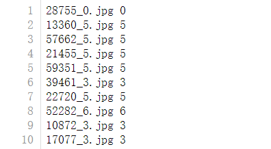
The file name of each jpg file corresponds to the actual number represented in this figure
The code is as follows:
#Example 4-1: Custom dataset - handwritten digits

import tensorflow as tf
from PIL import Image
import numpy as np
import os

#Training set picture path
train_path = './mnist_image_label/mnist_train_jpg_60000/'
#Training set label file
train_txt = './mnist_image_label/mnist_train_jpg_60000.txt'
#Training set input feature storage file
x_train_savepath = './mnist_image_label/mnist_x_train.npy'
#Training set label storage file
y_train_savepath = './mnist_image_label/mnist_y_train.npy'

#Test set picture path
test_path = './mnist_image_label/mnist_test_jpg_10000/'
#Test set label file
test_txt = './mnist_image_label/mnist_test_jpg_10000.txt'
#Test set input feature storage file
x_test_savepath = './mnist_image_label/mnist_x_test.npy'
#Test set label storage file
y_test_savepath = './mnist_image_label/mnist_y_test.npy'


#The custom generated function is used to customize the dataset
def generateds(path, txt):
    f = open(txt, 'r')  # Open txt file as read-only
    contents = f.readlines()  # Read all lines in the file
    f.close()  # Close txt file
    x, y_ = [], []  # Create an empty list
    for content in contents:  # Take out line by line
        value = content.split()  # Separated by spaces, the image path is value[0], and the label is value[1], which is stored in the list
        img_path = path + value[0]  # Spell out the picture path and file name
        img = Image.open(img_path)  # Read in picture
        img = np.array(img.convert('L'))  # The picture changes to NP with 8-bit wide gray value Array format
        img = img / 255.  # Data normalization (preprocessing)
        x.append(img)  # The normalized data is pasted to the list x
        y_.append(value[1])  # Label to list y_
        print('loading : ' + content)  # Print status prompt

    x = np.array(x)  # Becomes NP Array format
    y_ = np.array(y_)  # Becomes NP Array format
    y_ = y_.astype(np.int64)  # Change to 64 bit integer
    return x, y_  # Returns the input characteristic x and the label y_

#Judge whether the path and file exist. If they exist, read them directly. Otherwise, call the generated function to create the data set
if os.path.exists(x_train_savepath) and os.path.exists(y_train_savepath) and os.path.exists(
        x_test_savepath) and os.path.exists(y_test_savepath):
    print('-------------Load Datasets-----------------')
    x_train_save = np.load(x_train_savepath)
    y_train = np.load(y_train_savepath)
    x_test_save = np.load(x_test_savepath)
    y_test = np.load(y_test_savepath)
    x_train = np.reshape(x_train_save, (len(x_train_save), 28, 28))
    x_test = np.reshape(x_test_save, (len(x_test_save), 28, 28))
else:
    print('-------------Generate Datasets-----------------')
    x_train, y_train = generateds(train_path, train_txt)
    x_test, y_test = generateds(test_path, test_txt)

    print('-------------Save Datasets-----------------')
    x_train_save = np.reshape(x_train, (len(x_train), -1))
    x_test_save = np.reshape(x_test, (len(x_test), -1))
    np.save(x_train_savepath, x_train_save)
    np.save(y_train_savepath, y_train)
    np.save(x_test_savepath, x_test_save)
    np.save(y_test_savepath, y_test)

model = tf.keras.models.Sequential([
    tf.keras.layers.Flatten(),
    tf.keras.layers.Dense(128, activation='relu'),
    tf.keras.layers.Dense(10, activation='softmax')
])

model.compile(optimizer='adam',
              loss=tf.keras.losses.SparseCategoricalCrossentropy(from_logits=False),
              metrics=['sparse_categorical_accuracy'])

model.fit(x_train, y_train, batch_size=32, epochs=5, validation_data=(x_test, y_test), validation_freq=1)
model.summary()
4.2 data enhancement and expansion of data set
image_gen_train= tf.keras.preprocessing.image.ImageDataGenerator(
# use rescale to adjust the value of the input feature
rescale = all data will be multiplied by this value
# with rotation_range randomly rotates the angle of the image
rotation_range = random rotation angle range
# use width_shift_range randomly shifts the width of the image
width_shift_range = random width offset
# with height_shift_range performs random height offset on the image
height_shift_range = random height offset
# use horizontal_flip sets whether to flip horizontally at random
horizontal_flip = random horizontal flip
# use zoom_range randomly scales the image
zoom_range = range of random scaling [1-n,1+n]
)
image_gen_train.fit(x_train)
Or take the above custom dataset as an example to enhance the data of the custom dataset
#Example 4-2: data enhancement
#p11_show_augmented _images code
# Displays the original image and the enhanced image
import tensorflow as tf
from matplotlib import pyplot as plt
% matplotlib inline
from tensorflow.keras.preprocessing.image import ImageDataGenerator
import numpy as np

mnist = tf.keras.datasets.mnist
(x_train, y_train), (x_test, y_test) = mnist.load_data()
x_train = x_train.reshape(x_train.shape[0], 28, 28, 1)

image_gen_train = ImageDataGenerator(
    rescale=1. / 255,
    rotation_range=45,
    width_shift_range=.15,
    height_shift_range=.15,
    horizontal_flip=False,
    zoom_range=0.5
)
image_gen_train.fit(x_train)
print("xtrain",x_train.shape)
x_train_subset1 = np.squeeze(x_train[:12])
print("xtrain_subset1",x_train_subset1.shape)
print("xtrain",x_train.shape)
x_train_subset2 = x_train[:12]  # Display 12 pictures at a time
print("xtrain_subset2",x_train_subset2.shape)

fig = plt.figure(figsize=(20, 2))
plt.set_cmap('gray')
# Show original picture
for i in range(0, len(x_train_subset1)):
    ax = fig.add_subplot(1, 12, i + 1)
    ax.imshow(x_train_subset1[i])
fig.suptitle('Subset of Original Training Images', fontsize=20)
plt.show()

# Show enhanced pictures
fig = plt.figure(figsize=(20, 2))
for x_batch in image_gen_train.flow(x_train_subset2, batch_size=12, shuffle=False):
    for i in range(0, 12):
        ax = fig.add_subplot(1, 12, i + 1)
        ax.imshow(np.squeeze(x_batch[i]))
    fig.suptitle('Augmented Images', fontsize=20)
    plt.show()
    break;
4.3} continuous training
The model can be saved or read
load_ Weights (path file name)
Save model:
tf.keras.callbacks.ModelCheckpoint(
filepath = path file name
save_weights_only=True/False # whether to keep only model parameters
save_best_only=True/False # whether to keep only the optimal parameters
)
history=model.fit(callbacks=[cp_callback])
Take the above custom handwriting dataset as an example, and the code is as follows
#Example 4-3: breakpoint continuation training example
#p16_mnist_train_ex3
import tensorflow as tf
import os

mnist = tf.keras.datasets.mnist
(x_train, y_train), (x_test, y_test) = mnist.load_data()
x_train, x_test = x_train / 255.0, x_test / 255.0

model = tf.keras.models.Sequential([
    tf.keras.layers.Flatten(),
    tf.keras.layers.Dense(128, activation='relu'),
    tf.keras.layers.Dense(10, activation='softmax')
])

model.compile(optimizer='adam',
              loss=tf.keras.losses.SparseCategoricalCrossentropy(from_logits=False),
              metrics=['sparse_categorical_accuracy'])

checkpoint_save_path = "./checkpoint/mnist.ckpt"
if os.path.exists(checkpoint_save_path + '.index'):
    print('-------------load the model-----------------')
    model.load_weights(checkpoint_save_path)

cp_callback = tf.keras.callbacks.ModelCheckpoint(filepath=checkpoint_save_path,
                                                 save_weights_only=True,
                                                 save_best_only=True)

history = model.fit(x_train, y_train, batch_size=32, epochs=5, validation_data=(x_test, y_test), validation_freq=1,
                    callbacks=[cp_callback])
model.summary()
4.4} parameter extraction
model.trainable_variables returns the trainable parameters in the model
Set print output format
np.set_printoptions(threshold = how much more than is omitted)
np.set_printoptions(threshold=np.inf) #np. Inf means infinity, so the printed data will not have ellipsis
#Example 4-4: model parameter extraction
#p19_mnist_train_ex4 code
import tensorflow as tf
import os
import numpy as np
np.set_printoptions(threshold=np.inf)
mnist = tf.keras.datasets.mnist
(x_train, y_train), (x_test, y_test) = mnist.load_data()
x_train, x_test = x_train / 255.0, x_test / 255.0
model = tf.keras.models.Sequential([
    tf.keras.layers.Flatten(),
    tf.keras.layers.Dense(128, activation='relu'),
    tf.keras.layers.Dense(10, activation='softmax')
])
model.compile(optimizer='adam',
              loss=tf.keras.losses.SparseCategoricalCrossentropy(from_logits=False),
              metrics=['sparse_categorical_accuracy'])
checkpoint_save_path = "./checkpoint/mnist.ckpt"
if os.path.exists(checkpoint_save_path + '.index'):
    print('-------------load the model-----------------')
    model.load_weights(checkpoint_save_path)
cp_callback = tf.keras.callbacks.ModelCheckpoint(filepath=checkpoint_save_path,
                                                 save_weights_only=True,
                                                 save_best_only=True)
history = model.fit(x_train, y_train, batch_size=32, epochs=5, validation_data=(x_test, y_test), validation_freq=1,
                    callbacks=[cp_callback])
model.summary()
print(model.trainable_variables)
file = open('./weights.txt', 'w')
for v in model.trainable_variables:
    file.write(str(v.name) + '\n')
    file.write(str(v.shape) + '\n')
    file.write(str(v.numpy()) + '\n')
file.close()
4.5 acc curve and loss curve
#Example 4-5: visualization of training process
#p23_mnist_train_ex5
import tensorflow as tf
import os
import numpy as np
from matplotlib import pyplot as plt
% matplotlib inline

np.set_printoptions(threshold=np.inf)

mnist = tf.keras.datasets.mnist
(x_train, y_train), (x_test, y_test) = mnist.load_data()
x_train, x_test = x_train / 255.0, x_test / 255.0

model = tf.keras.models.Sequential([
    tf.keras.layers.Flatten(),
    tf.keras.layers.Dense(128, activation='relu'),
    tf.keras.layers.Dense(10, activation='softmax')
])

model.compile(optimizer='adam',
              loss=tf.keras.losses.SparseCategoricalCrossentropy(from_logits=False),
              metrics=['sparse_categorical_accuracy'])

checkpoint_save_path = "./checkpoint/mnist.ckpt"
if os.path.exists(checkpoint_save_path + '.index'):
    print('-------------load the model-----------------')
    model.load_weights(checkpoint_save_path)

cp_callback = tf.keras.callbacks.ModelCheckpoint(filepath=checkpoint_save_path,
                                                 save_weights_only=True,
                                                 save_best_only=True)

history = model.fit(x_train, y_train, batch_size=32, epochs=5, validation_data=(x_test, y_test), validation_freq=1,
                    callbacks=[cp_callback])
model.summary()

print(model.trainable_variables)
file = open('./weights.txt', 'w')
for v in model.trainable_variables:
    file.write(str(v.name) + '\n')
    file.write(str(v.shape) + '\n')
    file.write(str(v.numpy()) + '\n')
file.close()

###############################################    show   ###############################################

# Display acc and loss curves of training set and verification set
acc = history.history['sparse_categorical_accuracy']
val_acc = history.history['val_sparse_categorical_accuracy']
loss = history.history['loss']
val_loss = history.history['val_loss']

plt.subplot(1, 2, 1)
plt.plot(acc, label='Training Accuracy')
plt.plot(val_acc, label='Validation Accuracy')
plt.title('Training and Validation Accuracy')
plt.legend()

plt.subplot(1, 2, 2)
plt.plot(loss, label='Training Loss')
plt.plot(val_loss, label='Validation Loss')
plt.title('Training and Validation Loss')
plt.legend()
plt.show()
4.6 custom picture prediction
Predict (input characteristic, batch_size = integer) # returns the forward propagation calculation result
Reproduction model , model = TF keras. models. Sequential([
(forward propagation) TF keras. layers. Flatten(),
tf.keras.layers.Dense(128,activation='relu'),
tf.keras.layers.Dense(10,activation='softmax')]
)
Load parameter {model load_ weights(model_save_path)
Forecast result = model predict(x_predict)
#Example 4-6: custom picture prediction
from PIL import Image
import numpy as np
import tensorflow as tf

model_save_path = './checkpoint/mnist.ckpt'

model = tf.keras.models.Sequential([
    tf.keras.layers.Flatten(),
    tf.keras.layers.Dense(128, activation='relu'),
    tf.keras.layers.Dense(10, activation='softmax')])

model.load_weights(model_save_path)

preNum = int(input("input the number of test pictures:"))

for i in range(preNum):
    image_path = input("the path of test picture:")
    img = Image.open(image_path)
    img = img.resize((28, 28), Image.ANTIALIAS)
    img_arr = np.array(img.convert('L'))

    img_arr = 255 - img_arr

    img_arr = img_arr / 255.0
    print("img_arr:",img_arr.shape)
    x_predict = img_arr[tf.newaxis, ...]
    print("x_predict:",x_predict.shape)
    result = model.predict(x_predict)

    pred = tf.argmax(result, axis=1)

    print('\n')
    tf.print(pred)
5. Convolutional neural network
In practice, when processing the image, there are too many input parameters of the fully connected network, so the image features are generally extracted first, and then the extracted features are transmitted to the fully connected network for processing. Convolution calculation is an effective feature extraction method. Generally, a square convolution kernel is used to slide on the input feature map according to the specified step size, traverse each pixel of the input feature map, and for each step size, the convolution kernel will coincide with some pixels of the input feature map, multiply and sum the corresponding elements of the coincidence area, and add the offset term, Get a pixel of the output feature. The depth of the convolution kernel should be consistent with the depth of the input feature. The convolution kernel with depth of 1 is used for single channel gray image and 5 * 5 * 3 or 3 * 3 * 3 is used for 3-channel color image. Each convolution kernel generates a feature map, so the number of convolution kernels of the current layer determines the depth of the output feature map of the current layer. Convolution is the use of stereo convolution kernel to realize the spatial sharing of parameters.
5.1 convolution calculation process
5.2 receptive field
Receptive field refers to the area size of one pixel in the output feature map mapped to the original input picture
For example, for a 5 * 5 feature map, using a 3 * 3 convolution kernel will output a 3 * 3 output feature map. Each pixel on the output feature map is mapped to the area where the original picture is 3 * 3, so its receptive field is 3. If the convolution kernel of 5 * 5 is directly used for the characteristic graph of 5 * 5, a 1 * 1 output graph is obtained, so that the pixel receptive field of the 1 * 1 graph is 5.
The feature extraction ability of two-layer 3 * 3 convolution kernel is the same as that of a 5 * 5 convolution kernel.
However, the amount of parameters to be trained is different. The convolution kernel parameter quantity of 5 * 5 is 25, and the convolution kernel parameter quantity of two 3 * 3 is 18
The calculation amount of two layers of 3 * 3 is much smaller than that of one layer of 5 * 5
5.3 all zero filling
If we want the convolution calculation to keep the size of the input characteristic graph unchanged, we can use all 0 filling, that is, fill all the surrounding of the input characteristic graph with 0 before passing through the convolution kernel.
Full 0 filling: padding='same 'output graph side length = input length / step size (rounded up)
Incomplete 0 filling: padding='valid 'output graph side length = (input length - core length + 1) / step size (rounded up)
5.4 convolution function in TF
tf.keras.layers.Conv2D(
filters = number of convolution kernels
kernel_size = convolution kernel size, # square write kernel length integer, or (kernel height h, kernel width w)
Stripes = sliding step size, # horizontal and vertical same write step size integer, (or vertical step size h, horizontal step size w), default 1
Padding ='same 'or' valid ', # filling with all zeros is' same', not 'valid' (default)
Activation ='relu 'or' SIGMOD 'or' tanh 'or' softmax ', etc.
input_shape = (height, width, number of channels) # enter the dimension of the feature graph, which can be omitted
)
For example, the following is a three-layer convolution network
model=tf.keras.models.Sequential([
Conv2D(6,5,padding='valid',activation='sigmoid'),
MaxPool2D(2,2),
Conv2D(6,(5,5),padding='valid',activation='sigmoid'),
MaxPool2D(2,(2,2)),
Conv2D(filters=6,kernal_size=(5,5),padding='valid',activation='sigmoid'),
MaxPool2D(pool_size=(2,2),strides=2),
Flatten(),
Dense(10,activation='softmax')
])
5.5 standardization
Standardization refers to making the data conform to the standard normal distribution with 0 as the mean and 1 as the standard deviation.
Batch normalization (BN) is to standardize the data of a batch to make the data return to the standard normal distribution
Batch standardization is usually between convolution and activation operations
TF batch standardization function
tf.keras.layers.BatchNormalization()
model=tf.keras.models.Sequential([
Conv2D(filters=6,kernel_size=(5,5),padding='same'),
BatchNormalization(), #BN layer
Activation('relu '), # activate layer
Maxpool2d (pool_size = (2,2), stripes = 2, padding ='same '), # pool layer
Dropout(0,2), #dropout layer
])
5.6 pool operation
Pooling is used to reduce the amount of characteristic data.
Maximum pooling can extract image texture, and mean pooling can preserve background features
TF pooling function
tf.keras.layers.MaxPool2D(
pool_size = pool core size, # square write core length integer, or (core height h, core width w)
Stripes = pooled step size, # step size integer, or (vertical step size h, horizontal step size w). The default is pool_size
padding='valid 'or' same '# filling with all zeros is' same', not using is' valid '(default)
)
tf.keras.layers.AveragePooling2D(
pool_size = pool core size, # square write core length integer, or (core height h, core width w)
Stripes = pooled step size, # step size integer, or (vertical step size h, horizontal step size w). The default is pool_size
padding='valid 'or' same '# filling with all zeros is' same', not using is' valid '(default)
)
For example, the following is an example of maximum pooling
model=tf.keras.models.Sequential([
Conv2D(filters=6,kernel_size=(5,5),padding='same '), # convolution layer
BatchNormalization(), #BN layer
Activation('relu '), # activate layer
Maxpool2d (pool_size = (2,2), stripes = 2, padding ='same '), # pool layer
Dropout (0,2), #dropout layer
])
5.7 abandonment
In order to alleviate the over fitting of neural network, in neural network training, some neurons in the hidden layer are often temporarily discarded from the neural network according to a certain proportion, and all neurons are restored to the neural network when using the neural network
TF discard function
tf. keras. layer. Dropout (probability of abandonment)
model=tf.keras.models.Sequential([
Conv2D(filters=6,kernel_size=(5,5),padding='same '), # convolution layer
BatchNormalization(), #BN layer
Activation('relu '), # activate layer
MaxPool2D(pool_size=(2,2),strides=2,padding='same'),
Dropout(0,2), #dropout layer
])
5.8 general format of convolutional neural network
The so-called convolution neural network is to extract features with the help of convolution kernel and send them to the fully connected network for recognition and prediction
Feature extraction includes four steps: convolution, batch standardization, activation and pooling
Conv olution -- batch Standardization (BN) -- Activation -- Pooling -- full connection (FC)
model=tf.keras.models.Sequential([
Conv2D(filters=6,kernel_size=(5,5),padding='same '), # convolution layer
BatchNormalization(), #BN layer
Activation('relu '), # activate layer
MaxPool2D(pool_size=(2,2),strides=2,padding='same'),
Dropout(0,2), #dropout layer
])
5.9. Several commonly used convolutional neural networks
Take cifar10 data set as an example to demonstrate the usage of several common convolutional neural networks. Let's write the basic baseline code first
#5-1 convolutional neural network baseline code
import tensorflow as tf
import os
import numpy as np
from matplotlib import pyplot as plt
from tensorflow.keras.layers import Conv2D, BatchNormalization, Activation, MaxPool2D, Dropout, Flatten, Dense
from tensorflow.keras import Model

np.set_printoptions(threshold=np.inf)

cifar10 = tf.keras.datasets.cifar10
(x_train, y_train), (x_test, y_test) = cifar10.load_data()
x_train, x_test = x_train / 255.0, x_test / 255.0


class Baseline(Model):
    def __init__(self):
        super(Baseline, self).__init__()
        self.c1 = Conv2D(filters=6, kernel_size=(5, 5), padding='same')  # Convolution layer
        self.b1 = BatchNormalization()  # BN layer
        self.a1 = Activation('relu')  # Active layer
        self.p1 = MaxPool2D(pool_size=(2, 2), strides=2, padding='same')  # Pool layer
        self.d1 = Dropout(0.2)  # dropout layer

        self.flatten = Flatten()
        self.f1 = Dense(128, activation='relu')
        self.d2 = Dropout(0.2)
        self.f2 = Dense(10, activation='softmax')

    def call(self, x):
        x = self.c1(x)
        x = self.b1(x)
        x = self.a1(x)
        x = self.p1(x)
        x = self.d1(x)

        x = self.flatten(x)
        x = self.f1(x)
        x = self.d2(x)
        y = self.f2(x)
        return y


model = Baseline()

model.compile(optimizer='adam',
              loss=tf.keras.losses.SparseCategoricalCrossentropy(from_logits=False),
              metrics=['sparse_categorical_accuracy'])

checkpoint_save_path = "./checkpoint/Baseline.ckpt"
if os.path.exists(checkpoint_save_path + '.index'):
    print('-------------load the model-----------------')
    model.load_weights(checkpoint_save_path)

cp_callback = tf.keras.callbacks.ModelCheckpoint(filepath=checkpoint_save_path,
                                                 save_weights_only=True,
                                                 save_best_only=True)

history = model.fit(x_train, y_train, batch_size=32, epochs=5, validation_data=(x_test, y_test), validation_freq=1,
                    callbacks=[cp_callback])
model.summary()

# print(model.trainable_variables)
file = open('./weights.txt', 'w')
for v in model.trainable_variables:
    file.write(str(v.name) + '\n')
    file.write(str(v.shape) + '\n')
    file.write(str(v.numpy()) + '\n')
file.close()

###############################################    show   ###############################################

# Display acc and loss curves of training set and verification set
acc = history.history['sparse_categorical_accuracy']
val_acc = history.history['val_sparse_categorical_accuracy']
loss = history.history['loss']
val_loss = history.history['val_loss']

plt.subplot(1, 2, 1)
plt.plot(acc, label='Training Accuracy')
plt.plot(val_acc, label='Validation Accuracy')
plt.title('Training and Validation Accuracy')
plt.legend()

plt.subplot(1, 2, 2)
plt.plot(loss, label='Training Loss')
plt.plot(val_loss, label='Validation Loss')
plt.title('Training and Validation Loss')
plt.legend()
plt.show()
5.9.1. LeNet network
#Example 5-2 LetNet5 network example
import tensorflow as tf
import os
import numpy as np
from matplotlib import pyplot as plt
from tensorflow.keras.layers import Conv2D, BatchNormalization, Activation, MaxPool2D, Dropout, Flatten, Dense
from tensorflow.keras import Model

np.set_printoptions(threshold=np.inf)

cifar10 = tf.keras.datasets.cifar10
(x_train, y_train), (x_test, y_test) = cifar10.load_data()
x_train, x_test = x_train / 255.0, x_test / 255.0


class LeNet5(Model):
    def __init__(self):
        super(LeNet5, self).__init__()
        self.c1 = Conv2D(filters=6, kernel_size=(5, 5),
                         activation='sigmoid')
        self.p1 = MaxPool2D(pool_size=(2, 2), strides=2)

        self.c2 = Conv2D(filters=16, kernel_size=(5, 5),
                         activation='sigmoid')
        self.p2 = MaxPool2D(pool_size=(2, 2), strides=2)

        self.flatten = Flatten()
        self.f1 = Dense(120, activation='sigmoid')
        self.f2 = Dense(84, activation='sigmoid')
        self.f3 = Dense(10, activation='softmax')

    def call(self, x):
        x = self.c1(x)
        x = self.p1(x)

        x = self.c2(x)
        x = self.p2(x)

        x = self.flatten(x)
        x = self.f1(x)
        x = self.f2(x)
        y = self.f3(x)
        return y


model = LeNet5()

model.compile(optimizer='adam',
              loss=tf.keras.losses.SparseCategoricalCrossentropy(from_logits=False),
              metrics=['sparse_categorical_accuracy'])

checkpoint_save_path = "./checkpoint/LeNet5.ckpt"
if os.path.exists(checkpoint_save_path + '.index'):
    print('-------------load the model-----------------')
    model.load_weights(checkpoint_save_path)

cp_callback = tf.keras.callbacks.ModelCheckpoint(filepath=checkpoint_save_path,
                                                 save_weights_only=True,
                                                 save_best_only=True)

history = model.fit(x_train, y_train, batch_size=32, epochs=5, validation_data=(x_test, y_test), validation_freq=1,
                    callbacks=[cp_callback])
model.summary()

# print(model.trainable_variables)
file = open('./weights.txt', 'w')
for v in model.trainable_variables:
    file.write(str(v.name) + '\n')
    file.write(str(v.shape) + '\n')
    file.write(str(v.numpy()) + '\n')
file.close()

###############################################    show   ###############################################

# Display acc and loss curves of training set and verification set
acc = history.history['sparse_categorical_accuracy']
val_acc = history.history['val_sparse_categorical_accuracy']
loss = history.history['loss']
val_loss = history.history['val_loss']

plt.subplot(1, 2, 1)
plt.plot(acc, label='Training Accuracy')
plt.plot(val_acc, label='Validation Accuracy')
plt.title('Training and Validation Accuracy')
plt.legend()

plt.subplot(1, 2, 2)
plt.plot(loss, label='Training Loss')
plt.plot(val_loss, label='Validation Loss')
plt.title('Training and Validation Loss')
plt.legend()
plt.show()
5.9.2 AlexNet network
#Example 5-3 example of Alex Net8
import tensorflow as tf
import os
import numpy as np
from matplotlib import pyplot as plt
from tensorflow.keras.layers import Conv2D, BatchNormalization, Activation, MaxPool2D, Dropout, Flatten, Dense
from tensorflow.keras import Model

np.set_printoptions(threshold=np.inf)

cifar10 = tf.keras.datasets.cifar10
(x_train, y_train), (x_test, y_test) = cifar10.load_data()
x_train, x_test = x_train / 255.0, x_test / 255.0


class AlexNet8(Model):
    def __init__(self):
        super(AlexNet8, self).__init__()
        self.c1 = Conv2D(filters=96, kernel_size=(3, 3))
        self.b1 = BatchNormalization()
        self.a1 = Activation('relu')
        self.p1 = MaxPool2D(pool_size=(3, 3), strides=2)

        self.c2 = Conv2D(filters=256, kernel_size=(3, 3))
        self.b2 = BatchNormalization()
        self.a2 = Activation('relu')
        self.p2 = MaxPool2D(pool_size=(3, 3), strides=2)

        self.c3 = Conv2D(filters=384, kernel_size=(3, 3), padding='same',
                         activation='relu')

        self.c4 = Conv2D(filters=384, kernel_size=(3, 3), padding='same',
                         activation='relu')

        self.c5 = Conv2D(filters=256, kernel_size=(3, 3), padding='same',
                         activation='relu')
        self.p3 = MaxPool2D(pool_size=(3, 3), strides=2)

        self.flatten = Flatten()
        self.f1 = Dense(2048, activation='relu')
        self.d1 = Dropout(0.5)
        self.f2 = Dense(2048, activation='relu')
        self.d2 = Dropout(0.5)
        self.f3 = Dense(10, activation='softmax')

    def call(self, x):
        x = self.c1(x)
        x = self.b1(x)
        x = self.a1(x)
        x = self.p1(x)

        x = self.c2(x)
        x = self.b2(x)
        x = self.a2(x)
        x = self.p2(x)

        x = self.c3(x)

        x = self.c4(x)

        x = self.c5(x)
        x = self.p3(x)

        x = self.flatten(x)
        x = self.f1(x)
        x = self.d1(x)
        x = self.f2(x)
        x = self.d2(x)
        y = self.f3(x)
        return y


model = AlexNet8()

model.compile(optimizer='adam',
              loss=tf.keras.losses.SparseCategoricalCrossentropy(from_logits=False),
              metrics=['sparse_categorical_accuracy'])

checkpoint_save_path = "./checkpoint/AlexNet8.ckpt"
if os.path.exists(checkpoint_save_path + '.index'):
    print('-------------load the model-----------------')
    model.load_weights(checkpoint_save_path)

cp_callback = tf.keras.callbacks.ModelCheckpoint(filepath=checkpoint_save_path,
                                                 save_weights_only=True,
                                                 save_best_only=True)

history = model.fit(x_train, y_train, batch_size=32, epochs=5, validation_data=(x_test, y_test), validation_freq=1,
                    callbacks=[cp_callback])
model.summary()

# print(model.trainable_variables)
file = open('./weights.txt', 'w')
for v in model.trainable_variables:
    file.write(str(v.name) + '\n')
    file.write(str(v.shape) + '\n')
    file.write(str(v.numpy()) + '\n')
file.close()

###############################################    show   ###############################################

# Display acc and loss curves of training set and verification set
acc = history.history['sparse_categorical_accuracy']
val_acc = history.history['val_sparse_categorical_accuracy']
loss = history.history['loss']
val_loss = history.history['val_loss']

plt.subplot(1, 2, 1)
plt.plot(acc, label='Training Accuracy')
plt.plot(val_acc, label='Validation Accuracy')
plt.title('Training and Validation Accuracy')
plt.legend()

plt.subplot(1, 2, 2)
plt.plot(loss, label='Training Loss')
plt.plot(val_loss, label='Validation Loss')
plt.title('Training and Validation Loss')
plt.legend()
plt.show()
5.9.3 VGGNet network
#Example 5-4 VGGNet16 example
import tensorflow as tf
import os
import numpy as np
from matplotlib import pyplot as plt
from tensorflow.keras.layers import Conv2D, BatchNormalization, Activation, MaxPool2D, Dropout, Flatten, Dense
from tensorflow.keras import Model

np.set_printoptions(threshold=np.inf)

cifar10 = tf.keras.datasets.cifar10
(x_train, y_train), (x_test, y_test) = cifar10.load_data()
x_train, x_test = x_train / 255.0, x_test / 255.0


class VGG16(Model):
    def __init__(self):
        super(VGG16, self).__init__()
        self.c1 = Conv2D(filters=64, kernel_size=(3, 3), padding='same')  # Convolution layer 1
        self.b1 = BatchNormalization()  # BN layer 1
        self.a1 = Activation('relu')  # Activate layer 1
        self.c2 = Conv2D(filters=64, kernel_size=(3, 3), padding='same', )
        self.b2 = BatchNormalization()  # BN layer 1
        self.a2 = Activation('relu')  # Activate layer 1
        self.p1 = MaxPool2D(pool_size=(2, 2), strides=2, padding='same')
        self.d1 = Dropout(0.2)  # dropout layer

        self.c3 = Conv2D(filters=128, kernel_size=(3, 3), padding='same')
        self.b3 = BatchNormalization()  # BN layer 1
        self.a3 = Activation('relu')  # Activate layer 1
        self.c4 = Conv2D(filters=128, kernel_size=(3, 3), padding='same')
        self.b4 = BatchNormalization()  # BN layer 1
        self.a4 = Activation('relu')  # Activate layer 1
        self.p2 = MaxPool2D(pool_size=(2, 2), strides=2, padding='same')
        self.d2 = Dropout(0.2)  # dropout layer

        self.c5 = Conv2D(filters=256, kernel_size=(3, 3), padding='same')
        self.b5 = BatchNormalization()  # BN layer 1
        self.a5 = Activation('relu')  # Activate layer 1
        self.c6 = Conv2D(filters=256, kernel_size=(3, 3), padding='same')
        self.b6 = BatchNormalization()  # BN layer 1
        self.a6 = Activation('relu')  # Activate layer 1
        self.c7 = Conv2D(filters=256, kernel_size=(3, 3), padding='same')
        self.b7 = BatchNormalization()
        self.a7 = Activation('relu')
        self.p3 = MaxPool2D(pool_size=(2, 2), strides=2, padding='same')
        self.d3 = Dropout(0.2)

        self.c8 = Conv2D(filters=512, kernel_size=(3, 3), padding='same')
        self.b8 = BatchNormalization()  # BN layer 1
        self.a8 = Activation('relu')  # Activate layer 1
        self.c9 = Conv2D(filters=512, kernel_size=(3, 3), padding='same')
        self.b9 = BatchNormalization()  # BN layer 1
        self.a9 = Activation('relu')  # Activate layer 1
        self.c10 = Conv2D(filters=512, kernel_size=(3, 3), padding='same')
        self.b10 = BatchNormalization()
        self.a10 = Activation('relu')
        self.p4 = MaxPool2D(pool_size=(2, 2), strides=2, padding='same')
        self.d4 = Dropout(0.2)

        self.c11 = Conv2D(filters=512, kernel_size=(3, 3), padding='same')
        self.b11 = BatchNormalization()  # BN layer 1
        self.a11 = Activation('relu')  # Activate layer 1
        self.c12 = Conv2D(filters=512, kernel_size=(3, 3), padding='same')
        self.b12 = BatchNormalization()  # BN layer 1
        self.a12 = Activation('relu')  # Active layer 1
        self.c13 = Conv2D(filters=512, kernel_size=(3, 3), padding='same')
        self.b13 = BatchNormalization()
        self.a13 = Activation('relu')
        self.p5 = MaxPool2D(pool_size=(2, 2), strides=2, padding='same')
        self.d5 = Dropout(0.2)

        self.flatten = Flatten()
        self.f1 = Dense(512, activation='relu')
        self.d6 = Dropout(0.2)
        self.f2 = Dense(512, activation='relu')
        self.d7 = Dropout(0.2)
        self.f3 = Dense(10, activation='softmax')

    def call(self, x):
        x = self.c1(x)
        x = self.b1(x)
        x = self.a1(x)
        x = self.c2(x)
        x = self.b2(x)
        x = self.a2(x)
        x = self.p1(x)
        x = self.d1(x)

        x = self.c3(x)
        x = self.b3(x)
        x = self.a3(x)
        x = self.c4(x)
        x = self.b4(x)
        x = self.a4(x)
        x = self.p2(x)
        x = self.d2(x)

        x = self.c5(x)
        x = self.b5(x)
        x = self.a5(x)
        x = self.c6(x)
        x = self.b6(x)
        x = self.a6(x)
        x = self.c7(x)
        x = self.b7(x)
        x = self.a7(x)
        x = self.p3(x)
        x = self.d3(x)

        x = self.c8(x)
        x = self.b8(x)
        x = self.a8(x)
        x = self.c9(x)
        x = self.b9(x)
        x = self.a9(x)
        x = self.c10(x)
        x = self.b10(x)
        x = self.a10(x)
        x = self.p4(x)
        x = self.d4(x)

        x = self.c11(x)
        x = self.b11(x)
        x = self.a11(x)
        x = self.c12(x)
        x = self.b12(x)
        x = self.a12(x)
        x = self.c13(x)
        x = self.b13(x)
        x = self.a13(x)
        x = self.p5(x)
        x = self.d5(x)

        x = self.flatten(x)
        x = self.f1(x)
        x = self.d6(x)
        x = self.f2(x)
        x = self.d7(x)
        y = self.f3(x)
        return y


model = VGG16()

model.compile(optimizer='adam',
              loss=tf.keras.losses.SparseCategoricalCrossentropy(from_logits=False),
              metrics=['sparse_categorical_accuracy'])

checkpoint_save_path = "./checkpoint/VGG16.ckpt"
if os.path.exists(checkpoint_save_path + '.index'):
    print('-------------load the model-----------------')
    model.load_weights(checkpoint_save_path)

cp_callback = tf.keras.callbacks.ModelCheckpoint(filepath=checkpoint_save_path,
                                                 save_weights_only=True,
                                                 save_best_only=True)

history = model.fit(x_train, y_train, batch_size=32, epochs=5, validation_data=(x_test, y_test), validation_freq=1,
                    callbacks=[cp_callback])
model.summary()

# print(model.trainable_variables)
file = open('./weights.txt', 'w')
for v in model.trainable_variables:
    file.write(str(v.name) + '\n')
    file.write(str(v.shape) + '\n')
    file.write(str(v.numpy()) + '\n')
file.close()

###############################################    show   ###############################################

# Display acc and loss curves of training set and verification set
acc = history.history['sparse_categorical_accuracy']
val_acc = history.history['val_sparse_categorical_accuracy']
loss = history.history['loss']
val_loss = history.history['val_loss']

plt.subplot(1, 2, 1)
plt.plot(acc, label='Training Accuracy')
plt.plot(val_acc, label='Validation Accuracy')
plt.title('Training and Validation Accuracy')
plt.legend()

plt.subplot(1, 2, 2)
plt.plot(loss, label='Training Loss')
plt.plot(val_loss, label='Validation Loss')
plt.title('Training and Validation Loss')
plt.legend()
plt.show()
5.9.4. Inception net network
#Example 5-5 example of inception 10
import tensorflow as tf
import os
import numpy as np
from matplotlib import pyplot as plt
from tensorflow.keras.layers import Conv2D, BatchNormalization, Activation, MaxPool2D, Dropout, Flatten, Dense, \
    GlobalAveragePooling2D
from tensorflow.keras import Model

np.set_printoptions(threshold=np.inf)

cifar10 = tf.keras.datasets.cifar10
(x_train, y_train), (x_test, y_test) = cifar10.load_data()
x_train, x_test = x_train / 255.0, x_test / 255.0


class ConvBNRelu(Model):
    def __init__(self, ch, kernelsz=3, strides=1, padding='same'):
        super(ConvBNRelu, self).__init__()
        self.model = tf.keras.models.Sequential([
            Conv2D(ch, kernelsz, strides=strides, padding=padding),
            BatchNormalization(),
            Activation('relu')
        ])

    def call(self, x):
        x = self.model(x, training=False) #When training=False, BN calculates the mean and variance of the whole training set for batch normalization. When training=True, BN calculates the mean and variance of the current batch for batch normalization. When reasoning, training=False, the effect is good
        return x


class InceptionBlk(Model):
    def __init__(self, ch, strides=1):
        super(InceptionBlk, self).__init__()
        self.ch = ch
        self.strides = strides
        self.c1 = ConvBNRelu(ch, kernelsz=1, strides=strides)
        self.c2_1 = ConvBNRelu(ch, kernelsz=1, strides=strides)
        self.c2_2 = ConvBNRelu(ch, kernelsz=3, strides=1)
        self.c3_1 = ConvBNRelu(ch, kernelsz=1, strides=strides)
        self.c3_2 = ConvBNRelu(ch, kernelsz=5, strides=1)
        self.p4_1 = MaxPool2D(3, strides=1, padding='same')
        self.c4_2 = ConvBNRelu(ch, kernelsz=1, strides=strides)

    def call(self, x):
        x1 = self.c1(x)
        x2_1 = self.c2_1(x)
        x2_2 = self.c2_2(x2_1)
        x3_1 = self.c3_1(x)
        x3_2 = self.c3_2(x3_1)
        x4_1 = self.p4_1(x)
        x4_2 = self.c4_2(x4_1)
        # concat along axis=channel
        x = tf.concat([x1, x2_2, x3_2, x4_2], axis=3)
        return x


class Inception10(Model):
    def __init__(self, num_blocks, num_classes, init_ch=16, **kwargs):
        super(Inception10, self).__init__(**kwargs)
        self.in_channels = init_ch
        self.out_channels = init_ch
        self.num_blocks = num_blocks
        self.init_ch = init_ch
        self.c1 = ConvBNRelu(init_ch)
        self.blocks = tf.keras.models.Sequential()
        for block_id in range(num_blocks):
            for layer_id in range(2):
                if layer_id == 0:
                    block = InceptionBlk(self.out_channels, strides=2)
                else:
                    block = InceptionBlk(self.out_channels, strides=1)
                self.blocks.add(block)
            # enlarger out_channels per block
            self.out_channels *= 2
        self.p1 = GlobalAveragePooling2D()
        self.f1 = Dense(num_classes, activation='softmax')

    def call(self, x):
        x = self.c1(x)
        x = self.blocks(x)
        x = self.p1(x)
        y = self.f1(x)
        return y


model = Inception10(num_blocks=2, num_classes=10)

model.compile(optimizer='adam',
              loss=tf.keras.losses.SparseCategoricalCrossentropy(from_logits=False),
              metrics=['sparse_categorical_accuracy'])

checkpoint_save_path = "./checkpoint/Inception10.ckpt"
if os.path.exists(checkpoint_save_path + '.index'):
    print('-------------load the model-----------------')
    model.load_weights(checkpoint_save_path)

cp_callback = tf.keras.callbacks.ModelCheckpoint(filepath=checkpoint_save_path,
                                                 save_weights_only=True,
                                                 save_best_only=True)

history = model.fit(x_train, y_train, batch_size=32, epochs=5, validation_data=(x_test, y_test), validation_freq=1,
                    callbacks=[cp_callback])
model.summary()

# print(model.trainable_variables)
file = open('./weights.txt', 'w')
for v in model.trainable_variables:
    file.write(str(v.name) + '\n')
    file.write(str(v.shape) + '\n')
    file.write(str(v.numpy()) + '\n')
file.close()

###############################################    show   ###############################################

# Display acc and loss curves of training set and verification set
acc = history.history['sparse_categorical_accuracy']
val_acc = history.history['val_sparse_categorical_accuracy']
loss = history.history['loss']
val_loss = history.history['val_loss']

plt.subplot(1, 2, 1)
plt.plot(acc, label='Training Accuracy')
plt.plot(val_acc, label='Validation Accuracy')
plt.title('Training and Validation Accuracy')
plt.legend()

plt.subplot(1, 2, 2)
plt.plot(loss, label='Training Loss')
plt.plot(val_loss, label='Validation Loss')
plt.title('Training and Validation Loss')
plt.legend()
plt.show()
5.9.5 Resnet network
#Example 5-6 Resnet18 example
import tensorflow as tf
import os
import numpy as np
from matplotlib import pyplot as plt
from tensorflow.keras.layers import Conv2D, BatchNormalization, Activation, MaxPool2D, Dropout, Flatten, Dense
from tensorflow.keras import Model

np.set_printoptions(threshold=np.inf)

cifar10 = tf.keras.datasets.cifar10
(x_train, y_train), (x_test, y_test) = cifar10.load_data()
x_train, x_test = x_train / 255.0, x_test / 255.0


class ResnetBlock(Model):

    def __init__(self, filters, strides=1, residual_path=False):
        super(ResnetBlock, self).__init__()
        self.filters = filters
        self.strides = strides
        self.residual_path = residual_path

        self.c1 = Conv2D(filters, (3, 3), strides=strides, padding='same', use_bias=False)
        self.b1 = BatchNormalization()
        self.a1 = Activation('relu')

        self.c2 = Conv2D(filters, (3, 3), strides=1, padding='same', use_bias=False)
        self.b2 = BatchNormalization()

        # residual_ When path is True, down sample the input, that is, use 1x1 convolution kernel for convolution operation to ensure that X and F(x) dimensions are the same and can be added smoothly
        if residual_path:
            self.down_c1 = Conv2D(filters, (1, 1), strides=strides, padding='same', use_bias=False)
            self.down_b1 = BatchNormalization()

        self.a2 = Activation('relu')

    def call(self, inputs):
        residual = inputs  # Residual is equal to the input value itself, that is, residual=x
        # Calculate F(x) through convolution, BN layer and activation layer
        x = self.c1(inputs)
        x = self.b1(x)
        x = self.a1(x)

        x = self.c2(x)
        y = self.b2(x)

        if self.residual_path:
            residual = self.down_c1(inputs)
            residual = self.down_b1(residual)

        out = self.a2(y + residual)  # The final output is the sum of two parts, that is, F(x)+x or F(x)+Wx, and then activate the function
        return out


class ResNet18(Model):

    def __init__(self, block_list, initial_filters=64):  # block_list indicates that each block has several convolution layers
        super(ResNet18, self).__init__()
        self.num_blocks = len(block_list)  # How many block s are there
        self.block_list = block_list
        self.out_filters = initial_filters
        self.c1 = Conv2D(self.out_filters, (3, 3), strides=1, padding='same', use_bias=False)
        self.b1 = BatchNormalization()
        self.a1 = Activation('relu')
        self.blocks = tf.keras.models.Sequential()
        # Build ResNet network structure
        for block_id in range(len(block_list)):  # Which resnet block
            for layer_id in range(block_list[block_id]):  # Which convolution layer

                if block_id != 0 and layer_id == 0:  # Down sample the input of each block except the first block
                    block = ResnetBlock(self.out_filters, strides=2, residual_path=True)
                else:
                    block = ResnetBlock(self.out_filters, residual_path=False)
                self.blocks.add(block)  # Add the constructed block to resnet
            self.out_filters *= 2  # The number of convolution kernels of the next block is twice that of the previous block
        self.p1 = tf.keras.layers.GlobalAveragePooling2D()
        self.f1 = tf.keras.layers.Dense(10, activation='softmax', kernel_regularizer=tf.keras.regularizers.l2())

    def call(self, inputs):
        x = self.c1(inputs)
        x = self.b1(x)
        x = self.a1(x)
        x = self.blocks(x)
        x = self.p1(x)
        y = self.f1(x)
        return y


model = ResNet18([2, 2, 2, 2])

model.compile(optimizer='adam',
              loss=tf.keras.losses.SparseCategoricalCrossentropy(from_logits=False),
              metrics=['sparse_categorical_accuracy'])

checkpoint_save_path = "./checkpoint/ResNet18.ckpt"
if os.path.exists(checkpoint_save_path + '.index'):
    print('-------------load the model-----------------')
    model.load_weights(checkpoint_save_path)

cp_callback = tf.keras.callbacks.ModelCheckpoint(filepath=checkpoint_save_path,
                                                 save_weights_only=True,
                                                 save_best_only=True)

history = model.fit(x_train, y_train, batch_size=32, epochs=5, validation_data=(x_test, y_test), validation_freq=1,
                    callbacks=[cp_callback])
model.summary()

# print(model.trainable_variables)
file = open('./weights.txt', 'w')
for v in model.trainable_variables:
    file.write(str(v.name) + '\n')
    file.write(str(v.shape) + '\n')
    file.write(str(v.numpy()) + '\n')
file.close()

###############################################    show   ###############################################

# Display acc and loss curves of training set and verification set
acc = history.history['sparse_categorical_accuracy']
val_acc = history.history['val_sparse_categorical_accuracy']
loss = history.history['loss']
val_loss = history.history['val_loss']

plt.subplot(1, 2, 1)
plt.plot(acc, label='Training Accuracy')
plt.plot(val_acc, label='Validation Accuracy')
plt.title('Training and Validation Accuracy')
plt.legend()

plt.subplot(1, 2, 2)
plt.plot(loss, label='Training Loss')
plt.plot(val_loss, label='Validation Loss')
plt.title('Training and Validation Loss')
plt.legend()
plt.show()
6. Prediction of continuous data using cyclic neural network
Some data are related to time series and can be predicted from the above. At this time, the recurrent neural network RNN is used
6.1 circulating nuclear
The cyclic core is the memory, which is the basic unit of RNN.
The cyclic kernel has memory and realizes the information extraction of time series through the sharing of parameters at different times (three matrices Wxh, Whh, Why).
The following figure is a cyclic core with t states. The meaning of state t is time. ht is the state information stored in the memory at the current time, from h0 at time 0 to ht at time t.
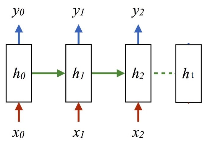
It can be understood as follows: a cyclic core has many layers. Each layer represents the state information ht at each time. ht at each time is updated until the last time ht is output to calculate our prediction Yt.
Xt: input feature
Yt: output characteristics
ht: status information stored in the memory at the current time (ht is refreshed at each time) Why, Whh, Wxh: three parameter matrices
Forward propagation: that is, when calculating HT and YT, the three matrices are fixed from beginning to end.
During back propagation: the three parameter matrices are updated by the gradient descent method (GD).
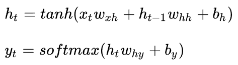
6.2 cycle nuclear time step deployment
Expanding according to the time step is to expand the cycle core according to the direction of the time axis. At each time, the memory state information ht is updated, and the parameter matrices wxh, whh and why around the memory are fixed. We train and optimize these parameter matrices. After the training, use the parameter matrix with the best effect to execute forward propagation and output the prediction results. In fact, This is consistent with our human prediction that the memory in your brain will be updated according to the current input. The current predictive reasoning is based on your previous knowledge accumulation and reasoning judgment with the solidified parameter matrix
Cyclic neural network: after extracting the time feature with the help of cyclic kernel, the extracted time feature information is sent to the fully connected network to realize the prediction of continuous data.
6.3 cycle calculation layer
Each loop core forms a loop computing layer. The number of layers of the loop computing layer increases in the direction of output. The number of memory in each loop core in each loop computing layer is arbitrarily specified according to your needs
6.4TF description cycle calculation layer
tf. keras. layers. Simplernn (number of memories, activation = 'activate function', return_sequences = whether to output ht to the next layer at each time)
activation = 'activate function' (do not write, use tanh by default)
return_sequences=True output ht of each time step
return_sequences=False output HT only in the last time step (default)
Example: SimpleRNN(3,return_sequences=True)
This api has requirements for the data dimension sent into the circulation layer, and the data sent into the circulation layer is required to be three-dimensional. The first dimension is the total number of samples sent in, the second dimension is the number of steps of the cyclic kernel expanded according to time steps, and the third dimension is the number of input features in each time step
Example: using circular network to realize letter prediction
Letter prediction: enter z to predict h, enter h to predict a, enter a to predict n, enter n to predict g, and enter g to predict z
z, h, a, n and g are coded as 10000, 01000, 00100, 00010 and 00001 by using the unique heat code
Then the unique hot codes of 'z', 'h', 'a', 'n' and 'g' are used as the training set x_train,
Take the unique hot codes of 'h', 'a', 'n', 'g' and 'z' as label y_train,
Then build an RNN network with 3 memories and a full connection layer. Because the output is only 5 letters, the parameter of density here is 5
Here is the complete code:
#Example 6-1 taking the string "zhang" as an example, a circular network is used to input one letter and predict the next letter
import numpy as np
import tensorflow as tf
from tensorflow.keras.layers import Dense, SimpleRNN
import matplotlib.pyplot as plt
import os

input_word = "zhang"
w_to_id = {'z': 0, 'h': 1, 'a': 2, 'n': 3, 'g': 4}  # Dictionary of words mapped to numeric IDS
id_to_onehot = {0: [1., 0., 0., 0., 0.], 1: [0., 1., 0., 0., 0.], 2: [0., 0., 1., 0., 0.], 3: [0., 0., 0., 1., 0.],
                4: [0., 0., 0., 0., 1.]}  # The id code is one hot

x_train = [id_to_onehot[w_to_id['z']], id_to_onehot[w_to_id['h']], id_to_onehot[w_to_id['a']],
           id_to_onehot[w_to_id['n']], id_to_onehot[w_to_id['g']]]
y_train = [w_to_id['h'], w_to_id['a'], w_to_id['n'], w_to_id['g'], w_to_id['z']]

np.random.seed(7)
np.random.shuffle(x_train)
np.random.seed(7)
np.random.shuffle(y_train)
tf.random.set_seed(7)

# Make x_ The train meets the input requirements of SimpleRNN: [the number of samples sent, the number of cycle kernel time expansion steps, and the number of features input in each time step].
# Here, the whole data set is sent, and the number of samples sent is len(x_train); Enter 1 letter to get the result, and the number of expansion steps of cycle kernel time is 1; It is expressed as a single hot code with 5 input features, and the number of input features in each time step is 5
x_train = np.reshape(x_train, (len(x_train), 1, 5))
y_train = np.array(y_train)

model = tf.keras.Sequential([
    SimpleRNN(3),
    Dense(5, activation='softmax')
])

model.compile(optimizer=tf.keras.optimizers.Adam(0.01),
              loss=tf.keras.losses.SparseCategoricalCrossentropy(from_logits=False),
              metrics=['sparse_categorical_accuracy'])

checkpoint_save_path = "./checkpoint/rnn_onehot_1pre1.ckpt"

if os.path.exists(checkpoint_save_path + '.index'):
    print('-------------load the model-----------------')
    model.load_weights(checkpoint_save_path)

cp_callback = tf.keras.callbacks.ModelCheckpoint(filepath=checkpoint_save_path,
                                                 save_weights_only=True,
                                                 save_best_only=True,
                                                 monitor='loss')  # Since fit does not give the test set, the accuracy of the test set is not calculated, and the optimal model is saved according to loss

history = model.fit(x_train, y_train, batch_size=32, epochs=100, callbacks=[cp_callback])

model.summary()

# print(model.trainable_variables)
file = open('./weights.txt', 'w')  # Parameter extraction
for v in model.trainable_variables:
    file.write(str(v.name) + '\n')
    file.write(str(v.shape) + '\n')
    file.write(str(v.numpy()) + '\n')
file.close()

###############################################    show   ###############################################

# Display acc and loss curves of training set and verification set
acc = history.history['sparse_categorical_accuracy']
loss = history.history['loss']

plt.subplot(1, 2, 1)
plt.plot(acc, label='Training Accuracy')
plt.title('Training Accuracy')
plt.legend()

plt.subplot(1, 2, 2)
plt.plot(loss, label='Training Loss')
plt.title('Training Loss')
plt.legend()
plt.show()

############### predict #############

preNum = int(input("Please enter the number of prediction letters:"))
for i in range(preNum):
    alphabet1 = input("Please enter the letter to predict:")
    alphabet = [id_to_onehot[w_to_id[alphabet1]]]
    # Make the alpha meet the input requirements of SimpleRNN: [the number of samples sent, the number of cycle kernel time expansion steps, and the number of features input in each time step]. Here, one sample is sent to verify the effect, and the number of samples sent is 1; Enter 1 letter to get the result, so the number of expansion steps of cycle kernel time is 1; It is expressed as a single hot code with 5 input features, and the number of input features in each time step is 5
    alphabet = np.reshape(alphabet, (1, 1, 5))
    result = model.predict([alphabet])
    pred = tf.argmax(result, axis=1)
    pred = int(pred)
    tf.print(alphabet1 + '->' + input_word[pred])
The following example shows how to input four letters continuously to get the prediction of the next letter
#Example 6-2 continuously input 4 letters to predict the next letter
import numpy as np
import tensorflow as tf
from tensorflow.keras.layers import Dense, SimpleRNN
import matplotlib.pyplot as plt
import os

input_word = "abcde"
w_to_id = {'a': 0, 'b': 1, 'c': 2, 'd': 3, 'e': 4}  # Dictionary of words mapped to numeric IDS
id_to_onehot = {0: [1., 0., 0., 0., 0.], 1: [0., 1., 0., 0., 0.], 2: [0., 0., 1., 0., 0.], 3: [0., 0., 0., 1., 0.],
                4: [0., 0., 0., 0., 1.]}  # The id code is one hot

x_train = [
    [id_to_onehot[w_to_id['a']], id_to_onehot[w_to_id['b']], id_to_onehot[w_to_id['c']], id_to_onehot[w_to_id['d']]],
    [id_to_onehot[w_to_id['b']], id_to_onehot[w_to_id['c']], id_to_onehot[w_to_id['d']], id_to_onehot[w_to_id['e']]],
    [id_to_onehot[w_to_id['c']], id_to_onehot[w_to_id['d']], id_to_onehot[w_to_id['e']], id_to_onehot[w_to_id['a']]],
    [id_to_onehot[w_to_id['d']], id_to_onehot[w_to_id['e']], id_to_onehot[w_to_id['a']], id_to_onehot[w_to_id['b']]],
    [id_to_onehot[w_to_id['e']], id_to_onehot[w_to_id['a']], id_to_onehot[w_to_id['b']], id_to_onehot[w_to_id['c']]],
]
y_train = [w_to_id['e'], w_to_id['a'], w_to_id['b'], w_to_id['c'], w_to_id['d']]

np.random.seed(7)
np.random.shuffle(x_train)
np.random.seed(7)
np.random.shuffle(y_train)
tf.random.set_seed(7)

# Make x_ The train meets the input requirements of SimpleRNN: [the number of samples sent, the number of cycle kernel time expansion steps, and the number of features input in each time step].
# Here, the whole data set is sent, and the number of samples sent is len(x_train); Input 4 letters to output the result, and the number of expansion steps of cycle kernel time is 4; It is expressed as a single hot code with 5 input features, and the number of input features in each time step is 5
x_train = np.reshape(x_train, (len(x_train), 4, 5))
y_train = np.array(y_train)

model = tf.keras.Sequential([
    SimpleRNN(3),
    Dense(5, activation='softmax')
])

model.compile(optimizer=tf.keras.optimizers.Adam(0.01),
              loss=tf.keras.losses.SparseCategoricalCrossentropy(from_logits=False),
              metrics=['sparse_categorical_accuracy'])

checkpoint_save_path = "./checkpoint/rnn_onehot_4pre1.ckpt"

if os.path.exists(checkpoint_save_path + '.index'):
    print('-------------load the model-----------------')
    model.load_weights(checkpoint_save_path)

cp_callback = tf.keras.callbacks.ModelCheckpoint(filepath=checkpoint_save_path,
                                                 save_weights_only=True,
                                                 save_best_only=True,
                                                 monitor='loss')  # Since fit does not give the test set, the accuracy of the test set is not calculated, and the optimal model is saved according to loss

history = model.fit(x_train, y_train, batch_size=32, epochs=100, callbacks=[cp_callback])

model.summary()

# print(model.trainable_variables)
file = open('./weights.txt', 'w')  # Parameter extraction
for v in model.trainable_variables:
    file.write(str(v.name) + '\n')
    file.write(str(v.shape) + '\n')
    file.write(str(v.numpy()) + '\n')
file.close()

###############################################    show   ###############################################

# Display acc and loss curves of training set and verification set
acc = history.history['sparse_categorical_accuracy']
loss = history.history['loss']

plt.subplot(1, 2, 1)
plt.plot(acc, label='Training Accuracy')
plt.title('Training Accuracy')
plt.legend()

plt.subplot(1, 2, 2)
plt.plot(loss, label='Training Loss')
plt.title('Training Loss')
plt.legend()
plt.show()

############### predict #############

preNum = int(input("input the number of test alphabet:"))
for i in range(preNum):
    alphabet1 = input("input test alphabet:")
    alphabet = [id_to_onehot[w_to_id[a]] for a in alphabet1]
    # Make the alpha meet the input requirements of SimpleRNN: [the number of samples sent, the number of cycle kernel time expansion steps, and the number of features input in each time step]. Here, one sample is sent to verify the effect, and the number of samples sent is 1; Enter 4 letters to get the result, so the number of expansion steps of cycle kernel time is 4; It is expressed as a single hot code with 5 input features, and the number of input features in each time step is 5
    alphabet = np.reshape(alphabet, (1, 4, 5))
    result = model.predict([alphabet])
    pred = tf.argmax(result, axis=1)
    pred = int(pred)
    tf.print(alphabet1 + '->' + input_word[pred])
6.5 Embedding , a coding method
Single hot code: the amount of data is large, too sparse, the mappings are independent, and there is no correlation
Embedding: it is a word coding method, which realizes the coding with low-dimensional vector. This coding is optimized through neural network training and can express the correlation between words.
tk. keras. layers. Embedding (vocabulary size, encoding dimension)
The coding dimension is to express a word with several numbers,
Example: TK keras. layers. Embedding(100,3)
It means to code 1-100. For example, the code of [4] is [0.25,0.1,0.11]
When entering Embedding, x_train dimension: [number of samples sent, cycle time, expansion steps]
#Example 6-3 using Embedding coding, RNN network can input four letters to predict the next letter
import numpy as np
import tensorflow as tf
from tensorflow.keras.layers import Dense, SimpleRNN, Embedding
import matplotlib.pyplot as plt
import os

input_word = "abcdefghijklmnopqrstuvwxyz"
w_to_id = {'a': 0, 'b': 1, 'c': 2, 'd': 3, 'e': 4,
           'f': 5, 'g': 6, 'h': 7, 'i': 8, 'j': 9,
           'k': 10, 'l': 11, 'm': 12, 'n': 13, 'o': 14,
           'p': 15, 'q': 16, 'r': 17, 's': 18, 't': 19,
           'u': 20, 'v': 21, 'w': 22, 'x': 23, 'y': 24, 'z': 25}  # Dictionary of words mapped to numeric IDS

training_set_scaled = [0, 1, 2, 3, 4, 5, 6, 7, 8, 9, 10,
                       11, 12, 13, 14, 15, 16, 17, 18, 19, 20,
                       21, 22, 23, 24, 25]

x_train = []
y_train = []

for i in range(4, 26):
    x_train.append(training_set_scaled[i - 4:i])
    y_train.append(training_set_scaled[i])

np.random.seed(7)
np.random.shuffle(x_train)
np.random.seed(7)
np.random.shuffle(y_train)
tf.random.set_seed(7)

# Make x_train meets the Embedding input requirements: [number of samples sent, cycle core time, expansion steps],
# Here, the whole data set is sent, and the number of samples sent is len(x_train); Enter 4 letters to get the result, and the number of expansion steps of cycle kernel time is 4.
x_train = np.reshape(x_train, (len(x_train), 4))
y_train = np.array(y_train)

model = tf.keras.Sequential([
    Embedding(26, 2),
    SimpleRNN(10),
    Dense(26, activation='softmax')
])

model.compile(optimizer=tf.keras.optimizers.Adam(0.01),
              loss=tf.keras.losses.SparseCategoricalCrossentropy(from_logits=False),
              metrics=['sparse_categorical_accuracy'])

checkpoint_save_path = "./checkpoint/rnn_embedding_4pre1.ckpt"

if os.path.exists(checkpoint_save_path + '.index'):
    print('-------------load the model-----------------')
    model.load_weights(checkpoint_save_path)

cp_callback = tf.keras.callbacks.ModelCheckpoint(filepath=checkpoint_save_path,
                                                 save_weights_only=True,
                                                 save_best_only=True,
                                                 monitor='loss')  # Since fit does not give the test set, the accuracy of the test set is not calculated, and the optimal model is saved according to loss

history = model.fit(x_train, y_train, batch_size=32, epochs=100, callbacks=[cp_callback])

model.summary()

file = open('./weights.txt', 'w')  # Parameter extraction
for v in model.trainable_variables:
    file.write(str(v.name) + '\n')
    file.write(str(v.shape) + '\n')
    file.write(str(v.numpy()) + '\n')
file.close()

###############################################    show   ###############################################

# Display acc and loss curves of training set and verification set
acc = history.history['sparse_categorical_accuracy']
loss = history.history['loss']

plt.subplot(1, 2, 1)
plt.plot(acc, label='Training Accuracy')
plt.title('Training Accuracy')
plt.legend()

plt.subplot(1, 2, 2)
plt.plot(loss, label='Training Loss')
plt.title('Training Loss')
plt.legend()
plt.show()

################# predict ##################

preNum = int(input("input the number of test alphabet:"))
for i in range(preNum):
    alphabet1 = input("input test alphabet:")
    alphabet = [w_to_id[a] for a in alphabet1]
    # Make the alpha meet the Embedding input requirements: [number of samples sent, time, expansion steps].
    # Here, one sample is sent to verify the effect, and the number of samples sent is 1; Enter 4 letters to get the result, and the number of expansion steps of cycle kernel time is 4.
    alphabet = np.reshape(alphabet, (1, 4))
    result = model.predict([alphabet])
    pred = tf.argmax(result, axis=1)
    pred = int(pred)
    tf.print(alphabet1 + '->' + input_word[pred])
6.6. Use RNN to realize the prediction of stock opening price
It should be noted here that there are too many factors affecting the stock price, and only simple processing is done here, so this prediction is unreliable, just to show that RNN can realize the prediction of continuous data. If you invest based on it, you will be responsible for the consequences.:)
It's just that there is this example in teacher Cao Jian's video course. Let's put it here as an example reference of RNN application.
First, we need to introduce a library tushare, which is a free and open source python financial data interface package. It mainly realizes the process of stock and other financial data from data collection, cleaning and processing to {data storage, which can provide financial analysts with fast, clean and diverse data convenient for analysis, greatly reduce their workload in data sources, and make them focus more on the research and implementation of strategies and models.
This is a necessary library for quantitative analysis. We use it to obtain the relevant data of a stock for a certain period of time. The code is as follows:
#Download stock data
import tushare as ts
import matplotlib.pyplot as plt

df1 = ts.get_k_data('600519', ktype='D', start='2010-04-26', end='2020-04-26')

datapath1 = "./SH600519.csv"
df1.to_csv(datapath1)
Among them, the 6-digit stock code can be changed into any stock you are interested in. Generally, SH is added in front of Shanghai stock market and SZ is added in front of Shenzhen stock market
Save it as a CSV file.
Then we use RNN network to predict the stock price
import numpy as np
import tensorflow as tf
from tensorflow.keras.layers import Dropout, Dense, SimpleRNN
import matplotlib.pyplot as plt
import os
import pandas as pd
from sklearn.preprocessing import MinMaxScaler
from sklearn.metrics import mean_squared_error, mean_absolute_error
import math

maotai = pd.read_csv('./SH600519.csv')  # Read stock file

training_set = maotai.iloc[0:2426 - 300, 2:3].values  # The opening price of the previous (2426-300 = 2126) days is used as the training set. The table counts from 0, and 2:3 is to extract [2:3) column, which is closed before opening, so the opening price of column C is extracted
test_set = maotai.iloc[2426 - 300:, 2:3].values  # The opening price after 300 days is used as the test set

# normalization
sc = MinMaxScaler(feature_range=(0, 1))  # Definition normalization: normalized to (0, 1)
training_set_scaled = sc.fit_transform(training_set)  # The maximum and minimum values of the training set are obtained, and the inherent attributes of these training sets are normalized on the training set
test_set = sc.transform(test_set)  # The test set is normalized by using the attributes of the training set

x_train = []
y_train = []

x_test = []
y_test = []

# Test set: data of the first 2426-300 = 2126 days in csv table
# The for loop is used to traverse the whole training set and extract the opening price of the training set for 60 consecutive days as the input feature x_train, the data on the 61st day is used as the label, and 2426-300-60 = 2066 groups of data are constructed in the for loop.
for i in range(60, len(training_set_scaled)):
    x_train.append(training_set_scaled[i - 60:i, 0])
    y_train.append(training_set_scaled[i, 0])
# Disrupt the training set
np.random.seed(7)
np.random.shuffle(x_train)
np.random.seed(7)
np.random.shuffle(y_train)
tf.random.set_seed(7)
# Change the training set from list format to array format
x_train, y_train = np.array(x_train), np.array(y_train)

# Make x_train meets the RNN input requirements: [number of samples sent, number of cycle kernel time expansion steps, and number of features input in each time step].
# Here, the whole data set is sent, and the number of samples sent is x_train.shape[0], i.e. 2066 sets of data; Input 60 opening prices, predict the opening price on the 61st day, and the number of steps of cycle verification time is 60; The input feature of each time step is the opening price of a day, and there is only one data, so the number of input features in each time step is 1
x_train = np.reshape(x_train, (x_train.shape[0], 60, 1))
# Test set: data of the last 300 days in csv table
# Use the for loop to traverse the whole test set, and extract the opening price of the test set for 60 consecutive days as the input feature x_train, the data on the 61st day is used as the label, and a total of 300-60 = 240 groups of data are constructed in the for loop.
for i in range(60, len(test_set)):
    x_test.append(test_set[i - 60:i, 0])
    y_test.append(test_set[i, 0])
# Test the set transformer array and reshape to meet the RNN input requirements: [the number of samples sent, the number of cycle kernel time expansion steps, and the number of input characteristics in each time step]
x_test, y_test = np.array(x_test), np.array(y_test)
x_test = np.reshape(x_test, (x_test.shape[0], 60, 1))

model = tf.keras.Sequential([
    SimpleRNN(80, return_sequences=True),
    Dropout(0.2),
    SimpleRNN(100),
    Dropout(0.2),
    Dense(1)
])

model.compile(optimizer=tf.keras.optimizers.Adam(0.001),
              loss='mean_squared_error')  # Mean square error for loss function
# The application only observes the loss value and does not observe the accuracy, so delete the metrics option and only display the loss value in each epoch iteration

checkpoint_save_path = "./checkpoint/rnn_stock.ckpt"

if os.path.exists(checkpoint_save_path + '.index'):
    print('-------------load the model-----------------')
    model.load_weights(checkpoint_save_path)

cp_callback = tf.keras.callbacks.ModelCheckpoint(filepath=checkpoint_save_path,
                                                 save_weights_only=True,
                                                 save_best_only=True,
                                                 monitor='val_loss')

history = model.fit(x_train, y_train, batch_size=64, epochs=50, validation_data=(x_test, y_test), validation_freq=1,
                    callbacks=[cp_callback])

model.summary()

file = open('./weights.txt', 'w')  # Parameter extraction
for v in model.trainable_variables:
    file.write(str(v.name) + '\n')
    file.write(str(v.shape) + '\n')
    file.write(str(v.numpy()) + '\n')
file.close()

loss = history.history['loss']
val_loss = history.history['val_loss']

plt.plot(loss, label='Training Loss')
plt.plot(val_loss, label='Validation Loss')
plt.title('Training and Validation Loss')
plt.legend()
plt.show()

################## predict ######################
# Test set input model for prediction
predicted_stock_price = model.predict(x_test)
# Restore the prediction data --- from (0, 1) inverse normalization to the original range
predicted_stock_price = sc.inverse_transform(predicted_stock_price)
# Restore real data --- from (0, 1) inverse normalization to original range
real_stock_price = sc.inverse_transform(test_set[60:])
# Draw the comparison curve between the real data and the predicted data
plt.plot(real_stock_price, color='red', label='Stock Price')
plt.plot(predicted_stock_price, color='blue', label='Predicted Stock Price')
plt.title('Stock Price Prediction')
plt.xlabel('Time')
plt.ylabel('Stock Price')
plt.legend()
plt.show()

##########evaluate##############
# calculate MSE mean square error -- > e [(predicted value - real value) ^ 2] (the predicted value minus the square of the real value to find the mean)
mse = mean_squared_error(predicted_stock_price, real_stock_price)
# calculate RMSE root mean square error -- > sqrt [MSE]
rmse = math.sqrt(mean_squared_error(predicted_stock_price, real_stock_price))
# calculate MAE mean absolute error ----- > e [| predicted value - true value |] (calculate the mean value after the predicted value minus the true value)
mae = mean_absolute_error(predicted_stock_price, real_stock_price)
print('Mean square error: %.6f' % mse)
print('Root mean square error: %.6f' % rmse)
print('Mean absolute error: %.6f' % mae)
Operation results:
#Omit the training process above
Epoch 49/50
33/33 [==============================] - 1s 28ms/step - loss: 0.0012 - val_loss: 0.0042
Epoch 50/50
33/33 [==============================] - 1s 25ms/step - loss: 0.0011 - val_loss: 0.0081
Model: "sequential"
_________________________________________________________________
 Layer (type)                Output Shape              Param #
=================================================================
 simple_rnn (SimpleRNN)      (None, 60, 80)            6560

 dropout (Dropout)           (None, 60, 80)            0

 simple_rnn_1 (SimpleRNN)    (None, 100)               18100

 dropout_1 (Dropout)         (None, 100)               0

 dense (Dense)               (None, 1)                 101

=================================================================
Total params: 24,761
Trainable params: 24,761
Non-trainable params: 0
_________________________________________________________________
Mean square error: 4064.279799
 Root mean square error: 63.751704
 Mean absolute error: 59.360308
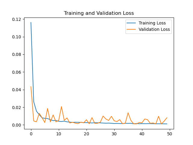
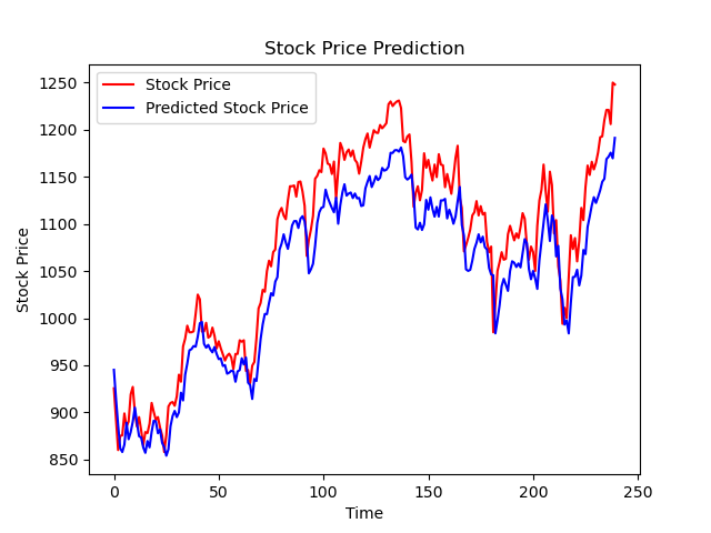
It seems pretty good. That's because China's stocks have a limit on the rise and fall of up to 10% every day, and most stocks have lower volatility. Then we use the data of the first 60 days to restrict, so the overall trend looks similar, but the actual prediction is not very accurate. Here we can only watch and play. We really want to be able to fight the stock, Then we should specialize in quantitative trading research.
6.7,LSTM
Long short term memory (LSTM) is a special RNN, which is mainly to solve the problems of gradient disappearance and gradient explosion in the process of long sequence training. In short, compared with ordinary RNN, LSTM can perform better in longer sequences.
The difference between LSTM and traditional RNN is shown in the figure below
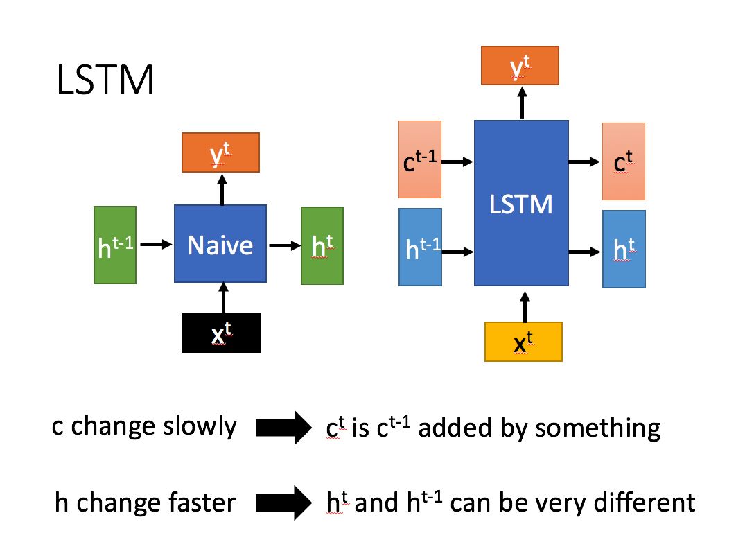
Compared with RNN with only one transmission state Ht, LSTM has two transmission states, one Ct (cell state) and one Ht (hidden state). (Tips: Ht in RNN for Ct in LSTM)
For the transmitted Ct , the change is very slow. Usually, the output Ct , is the Ct-1 , transmitted from the previous state plus some values.
However, Ht , is often very different under different nodes.
LSTM has three gates: input gate it, forgetting gate ft and output gate ot
Cell state Ct representing long-term memory, memory Ht representing short-term memory and candidate state Ct wave number waiting to be stored in long-term memory are also introduced
TF description LSTM layer:
tf. keras. layers. LSTM (number of memories, return_sequences = return output)
return_sequences=True = output Ht in each time step
return_sequences=False - output HT only in the last time step (default)
Let's use LSTM to predict the stock
import numpy as np
import tensorflow as tf
from tensorflow.keras.layers import Dropout, Dense, LSTM
import matplotlib.pyplot as plt
import os
import pandas as pd
from sklearn.preprocessing import MinMaxScaler
from sklearn.metrics import mean_squared_error, mean_absolute_error
import math

maotai = pd.read_csv('./SH600519.csv')  # Read stock file

training_set = maotai.iloc[0:2426 - 300, 2:3].values  # The opening price of the previous (2426-300 = 2126) days is used as the training set. The table counts from 0, and 2:3 is to extract [2:3) column, which is closed before opening, so the opening price of column C is extracted
test_set = maotai.iloc[2426 - 300:, 2:3].values  # The opening price after 300 days is used as the test set

# normalization
sc = MinMaxScaler(feature_range=(0, 1))  # Definition normalization: normalized to (0, 1)
training_set_scaled = sc.fit_transform(training_set)  # The maximum and minimum values of the training set are obtained, and the inherent attributes of these training sets are normalized on the training set
test_set = sc.transform(test_set)  # The test set is normalized by using the attributes of the training set

x_train = []
y_train = []

x_test = []
y_test = []

# Test set: data of the first 2426-300 = 2126 days in csv table
# The for loop is used to traverse the whole training set and extract the opening price of the training set for 60 consecutive days as the input feature x_train, the data on the 61st day is used as the label, and 2426-300-60 = 2066 groups of data are constructed in the for loop.
for i in range(60, len(training_set_scaled)):
    x_train.append(training_set_scaled[i - 60:i, 0])
    y_train.append(training_set_scaled[i, 0])
# Disrupt the training set
np.random.seed(7)
np.random.shuffle(x_train)
np.random.seed(7)
np.random.shuffle(y_train)
tf.random.set_seed(7)
# Change the training set from list format to array format
x_train, y_train = np.array(x_train), np.array(y_train)

# Make x_train meets the RNN input requirements: [number of samples sent, number of cycle kernel time expansion steps, and number of features input in each time step].
# Here, the whole data set is sent, and the number of samples sent is x_train.shape[0], i.e. 2066 sets of data; Input 60 opening prices, predict the opening price on the 61st day, and the number of steps of cycle verification time is 60; The input feature of each time step is the opening price of a day, and there is only one data, so the number of input features in each time step is 1
x_train = np.reshape(x_train, (x_train.shape[0], 60, 1))
# Test set: data of the last 300 days in csv table
# Use the for loop to traverse the whole test set, and extract the opening price of the test set for 60 consecutive days as the input feature x_train, the data on the 61st day is used as the label, and a total of 300-60 = 240 groups of data are constructed in the for loop.
for i in range(60, len(test_set)):
    x_test.append(test_set[i - 60:i, 0])
    y_test.append(test_set[i, 0])
# Test the set transformer array and reshape to meet the RNN input requirements: [the number of samples sent, the number of cycle kernel time expansion steps, and the number of input characteristics in each time step]
x_test, y_test = np.array(x_test), np.array(y_test)
x_test = np.reshape(x_test, (x_test.shape[0], 60, 1))

model = tf.keras.Sequential([
    LSTM(80, return_sequences=True),
    Dropout(0.2),
    LSTM(100),
    Dropout(0.2),
    Dense(1)
])

model.compile(optimizer=tf.keras.optimizers.Adam(0.001),
              loss='mean_squared_error')  # Mean square error for loss function
# The application only observes the loss value and does not observe the accuracy, so delete the metrics option and only display the loss value in each epoch iteration

checkpoint_save_path = "./checkpoint/LSTM_stock.ckpt"

if os.path.exists(checkpoint_save_path + '.index'):
    print('-------------load the model-----------------')
    model.load_weights(checkpoint_save_path)

cp_callback = tf.keras.callbacks.ModelCheckpoint(filepath=checkpoint_save_path,
                                                 save_weights_only=True,
                                                 save_best_only=True,
                                                 monitor='val_loss')

history = model.fit(x_train, y_train, batch_size=64, epochs=50, validation_data=(x_test, y_test), validation_freq=1,
                    callbacks=[cp_callback])

model.summary()

file = open('./weights.txt', 'w')  # Parameter extraction
for v in model.trainable_variables:
    file.write(str(v.name) + '\n')
    file.write(str(v.shape) + '\n')
    file.write(str(v.numpy()) + '\n')
file.close()

loss = history.history['loss']
val_loss = history.history['val_loss']

plt.plot(loss, label='Training Loss')
plt.plot(val_loss, label='Validation Loss')
plt.title('Training and Validation Loss')
plt.legend()
plt.show()

################## predict ######################
# Test set input model for prediction
predicted_stock_price = model.predict(x_test)
# Restore the prediction data --- from (0, 1) inverse normalization to the original range
predicted_stock_price = sc.inverse_transform(predicted_stock_price)
# Restore real data --- from (0, 1) inverse normalization to original range
real_stock_price = sc.inverse_transform(test_set[60:])
# Draw the comparison curve between the real data and the predicted data
plt.plot(real_stock_price, color='red', label='Stock Price')
plt.plot(predicted_stock_price, color='blue', label='Predicted Stock Price')
plt.title('Stock Price Prediction')
plt.xlabel('Time')
plt.ylabel('Stock Price')
plt.legend()
plt.show()

##########evaluate##############
# calculate MSE mean square error -- > e [(predicted value - real value) ^ 2] (the predicted value minus the square of the real value to find the mean)
mse = mean_squared_error(predicted_stock_price, real_stock_price)
# calculate RMSE root mean square error -- > sqrt [MSE]
rmse = math.sqrt(mean_squared_error(predicted_stock_price, real_stock_price))
# calculate MAE mean absolute error ----- > e [| predicted value - true value |] (calculate the mean value after the predicted value minus the true value)
mae = mean_absolute_error(predicted_stock_price, real_stock_price)
print('Mean square error: %.6f' % mse)
print('Root mean square error: %.6f' % rmse)
print('Mean absolute error: %.6f' % mae)
The result is not posted
6.8,GRU
GRU (Gate Recurrent Unit) is a kind of recurrent neural network (RNN). Like LSTM (long short term memory), it is also proposed to solve the problems of gradient in long-term memory and back propagation.
GRU and LSTM are almost the same in many cases. Why should we use GRU instead of LSTM?
In short, poverty limits our computing power
Compared with LSTM, using GRU can achieve considerable results, and it is easier to train, which can greatly improve the training efficiency. Therefore, it is more inclined to use GRU in many times.
TF description GRU layer:
tf. keras. layers. LSTM (number of memories, return_sequences = return output)
return_sequences=True = output Ht in each time step
return_sequences=False - output HT only in the last time step (default)
Next, use GRU to predict the stock:
import numpy as np
import tensorflow as tf
from tensorflow.keras.layers import Dropout, Dense, GRU
import matplotlib.pyplot as plt
import os
import pandas as pd
from sklearn.preprocessing import MinMaxScaler
from sklearn.metrics import mean_squared_error, mean_absolute_error
import math

maotai = pd.read_csv('./SH600519.csv')  # Read stock file

training_set = maotai.iloc[0:2426 - 300, 2:3].values  # The opening price of the previous (2426-300 = 2126) days is used as the training set. The table counts from 0, and 2:3 is to extract [2:3) column, which is closed before opening, so the opening price of column C is extracted
test_set = maotai.iloc[2426 - 300:, 2:3].values  # The opening price after 300 days is used as the test set

# normalization
sc = MinMaxScaler(feature_range=(0, 1))  # Definition normalization: normalized to (0, 1)
training_set_scaled = sc.fit_transform(training_set)  # The maximum and minimum values of the training set are obtained, and the inherent attributes of these training sets are normalized on the training set
test_set = sc.transform(test_set)  # The test set is normalized by using the attributes of the training set

x_train = []
y_train = []

x_test = []
y_test = []

# Test set: data of the first 2426-300 = 2126 days in csv table
# The for loop is used to traverse the whole training set and extract the opening price of the training set for 60 consecutive days as the input feature x_train, the data on the 61st day is used as the label, and 2426-300-60 = 2066 groups of data are constructed in the for loop.
for i in range(60, len(training_set_scaled)):
    x_train.append(training_set_scaled[i - 60:i, 0])
    y_train.append(training_set_scaled[i, 0])
# Disrupt the training set
np.random.seed(7)
np.random.shuffle(x_train)
np.random.seed(7)
np.random.shuffle(y_train)
tf.random.set_seed(7)
# Change the training set from list format to array format
x_train, y_train = np.array(x_train), np.array(y_train)

# Make x_train meets the RNN input requirements: [number of samples sent, number of cycle kernel time expansion steps, and number of features input in each time step].
# Here, the whole data set is sent, and the number of samples sent is x_train.shape[0], i.e. 2066 sets of data; Input 60 opening prices, predict the opening price on the 61st day, and the number of steps of cycle verification time is 60; The input feature of each time step is the opening price of a day, and there is only one data, so the number of input features in each time step is 1
x_train = np.reshape(x_train, (x_train.shape[0], 60, 1))
# Test set: data of the last 300 days in csv table
# Use the for loop to traverse the whole test set, and extract the opening price of the test set for 60 consecutive days as the input feature x_train, the data on the 61st day is used as the label, and a total of 300-60 = 240 groups of data are constructed in the for loop.
for i in range(60, len(test_set)):
    x_test.append(test_set[i - 60:i, 0])
    y_test.append(test_set[i, 0])
# Test the set transformer array and reshape to meet the RNN input requirements: [the number of samples sent, the number of cycle kernel time expansion steps, and the number of input characteristics in each time step]
x_test, y_test = np.array(x_test), np.array(y_test)
x_test = np.reshape(x_test, (x_test.shape[0], 60, 1))

model = tf.keras.Sequential([
    GRU(80, return_sequences=True),
    Dropout(0.2),
    GRU(100),
    Dropout(0.2),
    Dense(1)
])

model.compile(optimizer=tf.keras.optimizers.Adam(0.001),
              loss='mean_squared_error')  # Mean square error for loss function
# The application only observes the loss value and does not observe the accuracy, so delete the metrics option and only display the loss value in each epoch iteration

checkpoint_save_path = "./checkpoint/stock.ckpt"

if os.path.exists(checkpoint_save_path + '.index'):
    print('-------------load the model-----------------')
    model.load_weights(checkpoint_save_path)

cp_callback = tf.keras.callbacks.ModelCheckpoint(filepath=checkpoint_save_path,
                                                 save_weights_only=True,
                                                 save_best_only=True,
                                                 monitor='val_loss')

history = model.fit(x_train, y_train, batch_size=64, epochs=50, validation_data=(x_test, y_test), validation_freq=1,
                    callbacks=[cp_callback])

model.summary()

file = open('./weights.txt', 'w')  # Parameter extraction
for v in model.trainable_variables:
    file.write(str(v.name) + '\n')
    file.write(str(v.shape) + '\n')
    file.write(str(v.numpy()) + '\n')
file.close()

loss = history.history['loss']
val_loss = history.history['val_loss']

plt.plot(loss, label='Training Loss')
plt.plot(val_loss, label='Validation Loss')
plt.title('Training and Validation Loss')
plt.legend()
plt.show()

################## predict ######################
# Test set input model for prediction
predicted_stock_price = model.predict(x_test)
# Restore the prediction data --- from (0, 1) inverse normalization to the original range
predicted_stock_price = sc.inverse_transform(predicted_stock_price)
# Restore real data --- from (0, 1) inverse normalization to original range
real_stock_price = sc.inverse_transform(test_set[60:])
# Draw the comparison curve between the real data and the predicted data
plt.plot(real_stock_price, color='red', label='Stock Price')
plt.plot(predicted_stock_price, color='blue', label='Predicted Stock Price')
plt.title('Stock Price Prediction')
plt.xlabel('Time')
plt.ylabel('Stock Price')
plt.legend()
plt.show()

##########evaluate##############
# calculate MSE mean square error -- > e [(predicted value - real value) ^ 2] (the predicted value minus the square of the real value to find the mean)
mse = mean_squared_error(predicted_stock_price, real_stock_price)
# calculate RMSE root mean square error -- > sqrt [MSE]
rmse = math.sqrt(mean_squared_error(predicted_stock_price, real_stock_price))
# calculate MAE mean absolute error ----- > e [| predicted value - true value |] (calculate the mean value after the predicted value minus the true value)
mae = mean_absolute_error(predicted_stock_price, real_stock_price)
print('Mean square error: %.6f' % mse)
print('Root mean square error: %.6f' % rmse)
print('Mean absolute error: %.6f' % mae)
Prediction results:
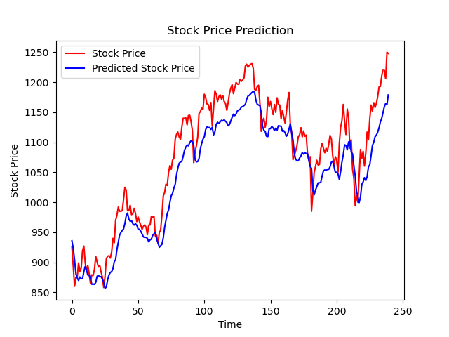
Ha ha, let's watch the result.
After learning this, TensorFlow is even an introduction. In the future, I will continue to learn how to use TensorFlow to solve specific AI problems, such as applications in the field of natural language processing (NLP), image classification, reinforcement learning, etc.