abstract
This example extracts part of the data in the plant seedling data set as the data set. The data set has 12 categories. Today, I work with you to implement tensorflow2 For the X version image classification task, the classification model uses MobileNetV3.
Through this article, you can learn:
1. Understand the characteristics of MobileNetV3.
2. How to load picture data and process data.
3. If the tag is converted to onehot code
4. How to use data enhancement.
5. How to use mixup.
6. How to segment data sets.
7. How to load the pre training model.
Introduction to mobilenetv3
MobileNetV3 was proposed by google team in 2019. It is the third version of mobilenet series. Its parameters are obtained by NAS (network architecture search). In ImageNet classification tasks, compared with V2, the accuracy increases by 3.2% and the calculation delay decreases by 20%. Deep separable convolution is proposed in V1, and V2 adds Linear Bottleneck and Inverted Residual on the basis of V1. What are the characteristics of V3?
Let's take a look at the network structure of v3. There are two versions of V3: Large and Small, which are applicable to different scenarios respectively. The network structure is as follows:
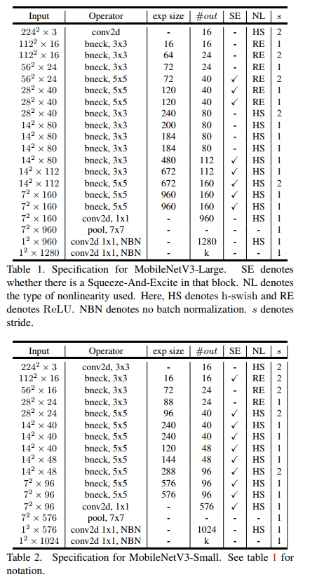
The above table shows the specific parameter settings, in which bneck is the basic structure of the network. SE represents whether channel attention mechanism is used. NL represents the type of activation function, including HS(h-swish),RE(ReLU). NBN means no BN operation. s means string. The network uses convolution string operation for downsampling instead of pooling operation.
Features of MobileNetV3:
- Inheriting the depth separable convolution of V1 and the residual structure with linear bottleneck of V2.
- The NetAdapt algorithm is used to obtain the optimal number of convolution cores and channels.
- A new activation function h-swish(x) is used to replace Relu6. Its formula is Relu6(x + 3)/6.
- The attention structure of Se channel is introduced, and Relu6(x + 3)/6 is used to approximate the sigmoid in SE module.
- The model is divided into Large and Small. In the ImageNet classification task, compared with V2, the Large accuracy rate increases by 3.2% and the calculation delay decreases by 20%.
Project structure
MobileNetV3_demo
├─data
│  ├─test
│  └─train
│      ├─Black-grass
│      ├─Charlock
│      ├─Cleavers
│      ├─Common Chickweed
│      ├─Common wheat
│      ├─Fat Hen
│      ├─Loose Silky-bent
│      ├─Maize
│      ├─Scentless Mayweed
│      ├─Shepherds Purse
│      ├─Small-flowered Cranesbill
│      └─Sugar beet
├─train.py
├─test1.py
└─test.py
train
1,Mixup
mixup is an unconventional data enhancement method, a simple data enhancement principle independent of data. It constructs new training samples and labels by linear interpolation. The final treatment of the tag is shown in the following formula, which is very simple, but it is very unusual for the enhancement strategy.

( x i , y i ) \left ( x_{i},y_{i} \right ) (xi,yi), ( x j , y j ) \left ( x_{j},y_{j} \right ) (xj, yj) two data pairs are training sample pairs (training samples and their corresponding labels) in the original data set. among λ \lambda λ Is a parameter subject to B distribution, λ ∼ B e t a ( α , α ) \lambda\sim Beta\left ( \alpha ,\alpha \right ) λ ∼Beta( α,α) . The probability density function of beta distribution is shown in the figure below, where α ∈ [ 0 , + ∞ ] \alpha \in \left [ 0,+\infty \right ] α∈[0,+∞]
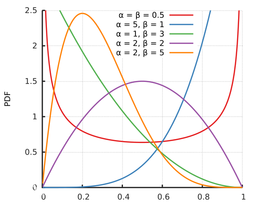
therefore α \alpha α Is a super parameter, with α \alpha α With the increase of, the training error of the network will increase, and its generalization ability will be enhanced. And when α → ∞ \alpha \rightarrow \infty α When →∞, the model will degenerate into the most primitive training strategy. reference resources: https://www.jianshu.com/p/d22fcd86f36d
Create a new mixupgenerator Py, insert the following code:
import numpy as np


class MixupGenerator():
    def __init__(self, X_train, y_train, batch_size=32, alpha=0.2, shuffle=True, datagen=None):
        self.X_train = X_train
        self.y_train = y_train
        self.batch_size = batch_size
        self.alpha = alpha
        self.shuffle = shuffle
        self.sample_num = len(X_train)
        self.datagen = datagen

    def __call__(self):
        while True:
            indexes = self.__get_exploration_order()
            itr_num = int(len(indexes) // (self.batch_size * 2))

            for i in range(itr_num):
                batch_ids = indexes[i * self.batch_size * 2:(i + 1) * self.batch_size * 2]
                X, y = self.__data_generation(batch_ids)

                yield X, y

    def __get_exploration_order(self):
        indexes = np.arange(self.sample_num)

        if self.shuffle:
            np.random.shuffle(indexes)

        return indexes

    def __data_generation(self, batch_ids):
        _, h, w, c = self.X_train.shape
        l = np.random.beta(self.alpha, self.alpha, self.batch_size)
        X_l = l.reshape(self.batch_size, 1, 1, 1)
        y_l = l.reshape(self.batch_size, 1)

        X1 = self.X_train[batch_ids[:self.batch_size]]
        X2 = self.X_train[batch_ids[self.batch_size:]]
        X = X1 * X_l + X2 * (1 - X_l)

        if self.datagen:
            for i in range(self.batch_size):
                X[i] = self.datagen.random_transform(X[i])
                X[i] = self.datagen.standardize(X[i])

        if isinstance(self.y_train, list):
            y = []

            for y_train_ in self.y_train:
                y1 = y_train_[batch_ids[:self.batch_size]]
                y2 = y_train_[batch_ids[self.batch_size:]]
                y.append(y1 * y_l + y2 * (1 - y_l))
        else:
            y1 = self.y_train[batch_ids[:self.batch_size]]
            y2 = self.y_train[batch_ids[self.batch_size:]]
            y = y1 * y_l + y2 * (1 - y_l)

        return X, y
2. Import the required data package and set the global parameters
import numpy as np
from tensorflow.keras.optimizers import Adam
import cv2
from tensorflow.keras.preprocessing.image import img_to_array
from sklearn.model_selection import train_test_split
from tensorflow.python.keras.callbacks import ModelCheckpoint, ReduceLROnPlateau
from tensorflow.keras.applications import MobileNetV3Large
import os

from tensorflow.python.keras.utils import np_utils
from tensorflow.python.keras.layers import Dense
from tensorflow.python.keras.models import Sequential

from mixupgenerator import MixupGenerator

norm_size = 224
datapath = 'data/train'
EPOCHS = 300
INIT_LR = 3e-4
labelList = []
dicClass = {'Black-grass': 0, 'Charlock': 1, 'Cleavers': 2, 'Common Chickweed': 3, 'Common wheat': 4, 'Fat Hen': 5, 'Loose Silky-bent': 6,
            'Maize': 7, 'Scentless Mayweed': 8, 'Shepherds Purse': 9, 'Small-flowered Cranesbill': 10, 'Sugar beet': 11}
classnum = 12
batch_size = 16
Here you can see tensorflow 2 Versions above 0 integrate keras. We don't need to install keras separately when using it. The previous code is upgraded to tensorflow2 For versions above 0, add tensorflow in front of keras.
After tensorflow is finished, let's explain some important global parameters:
-
norm_size = 224. The default image size of MobileNetV3 is 224 × 224.
-
datapath = 'data/train', set the path to store pictures. Here, it should be explained that if there are many pictures, they must not be placed in the project directory, otherwise pychar will browse all pictures when loading the project, which is very slow.
-
Epochs = 300. The number of epochs and the appropriate setting of epochs are very tangled. Generally, setting 300 is enough. If you feel that the training is not good, load the model for training.
-
INIT_LR = 3e-4, the learning rate generally decreases from 0.001 to 1e-6.
-
classnum = 12, the number of categories. There are 12 categories in the dataset. All of them define 12 categories.
-
batch_size = 16, batchsize. According to the hardware and the size of the data set, it is too small, the loss float is too large, and the convergence is not good. According to experience, it is generally set to the power of 2. windows can view the occupation of video memory through task manager.
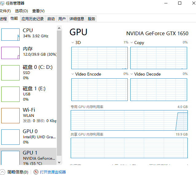
Ubuntu can use NVIDIA SMI to check the occupation of video memory.

3. Load picture
To process an image:
- Read image
- resize the image with the specified size.
- Convert image to array
- image normalization
- Use LabelBinarizer to convert labels to onehot encoding
See code for details:
def loadImageData():
    imageList = []
    listClasses = os.listdir(datapath)# Category folder
    for class_name in listClasses:
        class_path=os.path.join(datapath,class_name)
        image_names=os.listdir(class_path)
        for image_name in image_names:
            image_full_path = os.path.join(class_path, image_name)
            labelList.append(class_name)
            image = cv2.imdecode(np.fromfile(image_full_path, dtype=np.uint8), -1)
            image = cv2.resize(image, (norm_size, norm_size), interpolation=cv2.INTER_LANCZOS4)
            if image.shape[2] >3:
                image=image[:,:,:3]
                print(image.shape)
            image = img_to_array(image)
            imageList.append(image)
    imageList = np.array(imageList) / 255.0
    return imageList


print("Start loading data")
imageArr = loadImageData()
print("Loading data complete")
print(labelList)
lb = LabelBinarizer()
labelList = lb.fit_transform(labelList)
print(labelList)
print(lb.classes_)
f = open('label_bin.pickle', "wb")
f.write(pickle.dumps(lb))
f.close()
After making the data, we need to segment the training set and the test set, generally in the proportion of 4:1 or 7:3. Split dataset using train_test_split() method, import from sklearn model_ selection import train_ test_ Split package. Example:
trainX, valX, trainY, valY = train_test_split(imageArr, labelList, test_size=0.2, random_state=42)
4. Image enhancement
ImageDataGenerator() is keras preprocessing. The image generator in the image module can also enhance the data in batch, expand the size of the data set and enhance the generalization ability of the model. Such as rotation, deformation, normalization and so on.
keras.preprocessing.image.ImageDataGenerator(featurewise_center=False,samplewise_center
=False, featurewise_std_normalization=False, samplewise_std_normalization=False,zca_whitening=False,
 zca_epsilon=1e-06, rotation_range=0.0, width_shift_range=0.0, height_shift_range=0.0,brightness_range=None, shear_range=0.0, zoom_range=0.0,channel_shift_range=0.0, fill_mode='nearest', cval=0.0, horizontal_flip=False, vertical_flip=False, rescale=None, preprocessing_function=None,data_format=None,validation_split=0.0)
Parameters:
- featurewise_center: Boolean. Subtract the corresponding mean value of each channel from each channel of the input picture.
- samplewise_center: Boolan. Subtract the sample mean from each picture so that the sample mean is 0.
- featurewise_std_normalization(): Boolean()
- samplewise_std_normalization(): Boolean()
- zca_epsilon(): Default 12-6
- zca_whitening: Boolean. Removal of correlation between samples
- rotation_range(): rotation range
- width_shift_range(): horizontal translation range
- height_shift_range(): vertical translation range
- shear_range(): float, the range of perspective transformation
- zoom_range(): zoom range
- fill_mode: fill mode, constant, closest, reflect
- cval: fill_ 'constant mode ='
- horizontal_flip(): horizontal reversal
- vertical_flip(): flip vertically
- preprocessing_ Function (): processing function provided by user
- data_format(): channels_first or channels_last
- validation_split(): how much data is used to validate the set
The image enhancement code used in this example is as follows:
from tensorflow.keras.preprocessing.image import ImageDataGenerator

train_datagen = ImageDataGenerator(
                                   rotation_range=20,
                                   width_shift_range=0.2,
                                   height_shift_range=0.2,
                                   horizontal_flip=True)
val_datagen = ImageDataGenerator()  # The verification set does not do image enhancement
training_generator_mix = MixupGenerator(trainX, trainY, batch_size=batch_size, alpha=0.2, datagen=train_datagen)()
val_generator = val_datagen.flow(valX, valY, batch_size=batch_size, shuffle=True)
Note: only the training set is enhanced, not the verification set.
5. Keep the best model and dynamically set the learning rate
Model checkpoint: used to save the best model.
The syntax is as follows:
keras.callbacks.ModelCheckpoint(filepath, monitor='val_loss', verbose=0, save_best_only=False, save_weights_only=False, mode='auto', period=1)
The callback function will save the model to filepath after each epoch
filepath can be a formatted string, and the placeholder inside will be passed in by the epoch value and on_ epoch_ The logs keyword of end
For example, if filepath is weights {epoch:02d-{val_loss:.2f}}. HDF5, multiple files corresponding to epoch and verification set loss will be generated.
parameter
- filename: string, the path to save the model
- monitor: the value to be monitored
- verbose: information display mode, 0 or 1
- save_best_only: when set to True, only the best performing models on the validation set will be saved
- Mode: one of 'auto', 'min' and 'Max', in save_ best_ When only = true, it determines the evaluation criteria of the best performance model, for example, when the monitoring value is val_acc, the mode should be max, when the detection value is val_ When loss, the mode should be min. In auto mode, the evaluation criteria are automatically inferred from the name of the monitored value.
- save_weights_only: if it is set to True, only the model weight will be saved, otherwise the whole model (including model structure, configuration information, etc.) will be saved
- period: the number of epoch s in the interval between checkpoints
Reducerlonplateau: when the evaluation index is not improving, reduce the learning rate. The syntax is as follows:
keras.callbacks.ReduceLROnPlateau(monitor='val_loss', factor=0.1, patience=10, verbose=0, mode='auto', epsilon=0.0001, cooldown=0, min_lr=0)
When learning stagnates, reducing the learning rate by 2 or 10 times can often achieve better results. This callback function detects the condition of the index. If the performance improvement of the model is not seen in the patient epoch s, the learning rate will be reduced
parameter
- monitor: monitored quantity
- Factor: the factor that reduces the learning rate each time. The learning rate will be reduced in the form of lr = lr*factor
- patience: when an epoch passes and the performance of the model does not improve, the action of reducing the learning rate will be triggered
- Mode: 'auto', 'min' and 'max'. In Min mode, if the detection value triggers the reduction of learning rate. In max mode, when the detection value no longer rises, the learning rate decreases.
- epsilon: threshold, used to determine whether to enter the "plain area" of the detection value
- Cooldown: after the learning rate decreases, the normal operation will be resumed after a cooldown epoch
- min_lr: lower limit of learning rate
The code of this example is as follows:
checkpointer = ModelCheckpoint(filepath='best_model.hdf5',
                               monitor='val_accuracy', verbose=1, save_best_only=True, mode='max')

reduce = ReduceLROnPlateau(monitor='val_accuracy', patience=10,
                           verbose=1,
                           factor=0.5,
                           min_lr=1e-6)
6. Modeling and training
model = Sequential()
model.add(MobileNetV3Large(input_shape=(224,224,3),include_top=False, pooling='avg', weights='imagenet'))
model.add(Dense(classnum, activation='softmax'))
model.summary()
optimizer = Adam(learning_rate=INIT_LR)
model.compile(optimizer=optimizer, loss='categorical_crossentropy', metrics=['accuracy'])

history = model.fit(training_generator_mix,
                              steps_per_epoch=trainX.shape[0] / batch_size,
                              validation_data=val_generator,
                              epochs=EPOCHS,
                              validation_steps=valX.shape[0] / batch_size,
                              callbacks=[checkpointer, reduce])
model.save('my_model.h5')
print("[INFO] evaluating network...")
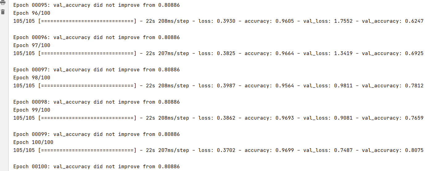
Operation results:
300 epoch s have been trained, and the accuracy has reached 0.80.
7. Model evaluation
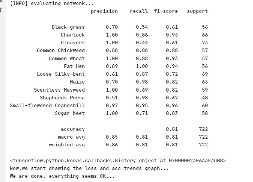
Using classification_report evaluates the validation set and imports the package from sklearn metrics import classification_report
predictions = model.predict(x=valX, batch_size=16)
print(classification_report(valY.argmax(axis=1),
	predictions.argmax(axis=1), target_names=lb.classes_))
The operation results are as follows:
8. Keep the training results and generate pictures
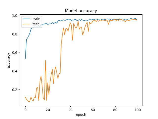
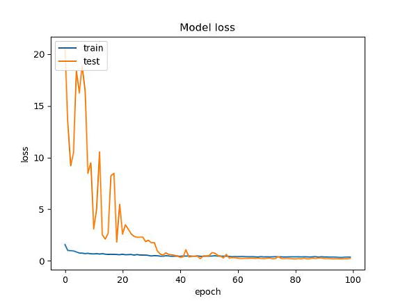
loss_trend_graph_path = r"WW_loss.jpg"
acc_trend_graph_path = r"WW_acc.jpg"
import matplotlib.pyplot as plt

print("Now,we start drawing the loss and acc trends graph...")
# summarize history for accuracy
fig = plt.figure(1)
plt.plot(history.history["accuracy"])
plt.plot(history.history["val_accuracy"])
plt.title("Model accuracy")
plt.ylabel("accuracy")
plt.xlabel("epoch")
plt.legend(["train", "test"], loc="upper left")
plt.savefig(acc_trend_graph_path)
plt.close(1)
# summarize history for loss
fig = plt.figure(2)
plt.plot(history.history["loss"])
plt.plot(history.history["val_loss"])
plt.title("Model loss")
plt.ylabel("loss")
plt.xlabel("epoch")
plt.legend(["train", "test"], loc="upper left")
plt.savefig(loss_trend_graph_path)
plt.close(2)
print("We are done, everything seems OK...")
# #windows system setting 10 shutdown
#os.system("shutdown -s -t 10")
result:
Test part
Single picture prediction
1. Import dependency
import pickle
import cv2
import numpy as np
from tensorflow.keras.preprocessing.image import img_to_array
from  tensorflow.keras.models import load_model
import time
2. Set global parameters
Note here that the order of the dictionary is consistent with that of the training
norm_size=224
imagelist=[]
emotion_labels = {
    0: 'Black-grass',
    1: 'Charlock',
    2: 'Cleavers',
    3: 'Common Chickweed',
    4: 'Common wheat',
    5: 'Fat Hen',
    6: 'Loose Silky-bent',
    7: 'Maize',
    8: 'Scentless Mayweed',
    9: 'Shepherds Purse',
    10: 'Small-flowered Cranesbill',
    11: 'Sugar beet',
}
3. Loading model
Here we need to load two models, one is LabelBinarizer model and the other is MobileNetV3Large model.
emotion_classifier=load_model("best_model.hdf5")
lb = pickle.loads(open("label_bin.pickle", "rb").read())
t1=time.time()
4. Processing pictures
The logic of processing pictures is similar to that of training sets. The steps are as follows:
- Read picture
- resize the picture to norm_size × norm_size.
- Convert the picture to an array.
- Put it in the imagelist.
- Divide the whole imagelist by 255 and scale the value to between 0 and 1.
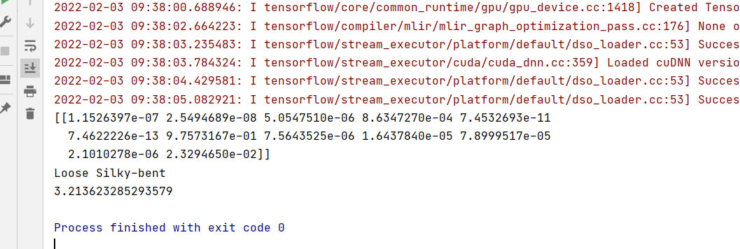
image = cv2.imdecode(np.fromfile('data/test/0a64e3e6c.png', dtype=np.uint8), -1)
# load the image, pre-process it, and store it in the data list
image = cv2.resize(image, (norm_size, norm_size), interpolation=cv2.INTER_LANCZOS4)
image = img_to_array(image)
imagelist.append(image)
imageList = np.array(imagelist, dtype="float") / 255.0
5. Forecast category
Predict the category and get the index of the highest category.
out=emotion_classifier.predict(imageList)
print(out)
pre=np.argmax(out)
label = lb.classes_[pre]
t2=time.time()
print(label)
t3=t2-t1
print(t3)
Operation results:
Batch forecast
The difference between batch forecast and single forecast is mainly in reading data and processing of forecast category after the forecast is completed. Nothing else has changed.
Steps:
- Load the model.
- Define the directory of the test set
- Get pictures in the directory
- Loop picture
- Read picture
- resize picture
- Turn array
- Put it in imageList
- Zoom to 0 to 255
- forecast
emotion_classifier=load_model("best_model.hdf5")
lb = pickle.loads(open("label_bin.pickle", "rb").read())
t1=time.time()
predict_dir = 'data/test'
test11 = os.listdir(predict_dir)
for file in test11:
    filepath=os.path.join(predict_dir,file)

    image = cv2.imdecode(np.fromfile(filepath, dtype=np.uint8), -1)
    # load the image, pre-process it, and store it in the data list
    image = cv2.resize(image, (norm_size, norm_size), interpolation=cv2.INTER_LANCZOS4)
    image = img_to_array(image)
    imagelist.append(image)
imageList = np.array(imagelist, dtype="float") / 255.0
out = emotion_classifier.predict(imageList)
print(out)
pre = [np.argmax(i) for i in out]
class_name_list=[lb.classes_[i] for i in pre]
print(class_name_list)
t2 = time.time()
t3 = t2 - t1
print(t3)
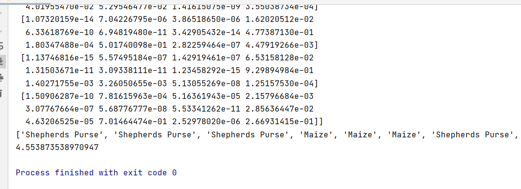
Operation results:
Full code: