Test Data for Trading - sentimental Analysis series articles explain the contents of Chapter 14 of machine learning for ethical trading and reproduce relevant codes. Because there are great differences between Chinese and English text analysis, this series does not select the materials in the Chinese market as the data of code reproduction, but selects the source code behind the book for reproduction.
From token to number: document term matrix
The word bag model represents a document according to the frequency of terms or tags it contains. Each document is a vector, and each tag in the vocabulary has an entry, reflecting the relevance of the tag to the document.
In view of the existence of vocabulary, the document term matrix can be calculated directly. However, it is also a rough simplification because it abstracts the relationship between word order and grammar. Nevertheless, it can often achieve good results quickly in text classification, so it is a very useful starting point.
There are several ways to weigh a tagged vector entry to capture its relevance to the file. We will explain how to use sklearn to use binary flags, counts and weighted counts indicating presence or absence. These counts take into account the differences in the frequency of terms in all documents, that is, in the corpus.
#Introduce some required libraries and packages to build the environment
from collections import Counter
from pathlib import Path
import numpy as np
import pandas as pd
from scipy import sparse
from scipy.spatial.distance import pdist
import matplotlib.pyplot as plt
from matplotlib.ticker import ScalarFormatter
import seaborn as sns
from ipywidgets import interact, FloatRangeSlider
import spacy
from sklearn.feature_extraction.text import CountVectorizer, TfidfVectorizer, TfidfTransformer
from sklearn.model_selection import train_test_split
Import the bbc data mentioned in the previous sections
#Convert data to dataframe format
docs = pd.DataFrame(doc_list, columns=['topic', 'heading', 'body'])
docs.info()
Inspection results
docs.sample(10)
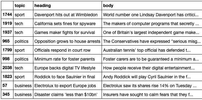 BBC data is extracted from five texts.
#Get the proportion of five categories in bbc data
docs.topic.value_counts(normalize=True).to_frame('count').style.format({'count': '{:,.2%}'.format})
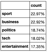 The proportions of the five types of text in the resulting bbc document are shown in the figure.
1. Count tokens
#Calculate the number of word s in the whole corpus
word_count = docs.body.str.split().str.len().sum()
print(f'Total word count: {word_count:,d} | per article: {word_count/len(docs):,.0f}')
#There are 842910 word s in total
Total word count: 842,910 | per article: 379
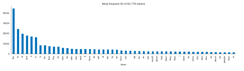
2. Count the 50 token s with the highest frequency
token_count = Counter()
for i, doc in enumerate(docs.body.tolist(), 1):
    if i % 500 == 0:
        print(i, end=' ', flush=True)
    token_count.update([t.strip() for t in
n = 50
(tokens
 .iloc[:50]
 .plot
 .bar(figsize=(14, 4), title=f'Most frequent {n} of {len(tokens):,d} tokens'))
sns.despine()
plt.tight_layout();
#50 token s with the highest frequency are detected and visualized
 3. Generate document - term matrix using CountVectorizer
The scikit learn preprocessing module provides two tools to create a document term matrix. The CountVectorizer uses binary or absolute counts to measure the term frequency tf (d, t) of each document d and token t.
Instead, TfIDFVectorizer measures (absolute) term frequency with inverse document frequency (idf). In other words, a term that appears in more documents will get lower weight.
The TF IDF vector of each document is normalized. TF IDF measure was originally used for information retrieval and ranking the results of search engines. Later, it was found to be very useful for text classification or clustering.
The key parameters affecting vocabulary size are:
stop_words: use a built-in or provide a list of (frequent) words to exclude (such as and, the)
ngram_range: n-grams in the N range defined by the (nmin, nmax) tuple.
max_features: limit the number of tags in the glossary accordingly
4. Document frequency distribution
binary_vectorizer = CountVectorizer(max_df=1.0,
                                    min_df=1,
                                    binary=True)

binary_dtm = binary_vectorizer.fit_transform(docs.body)
binary_dtm
n_docs, n_tokens = binary_dtm.shape
tokens_dtm = binary_vectorizer.get_feature_names()
5,min_df and max_df - interactive visualization
This paragraph discusses min_df and Max_ The influence of DF setting on vocabulary size. Read the document into a DataFrame, set CountVectorizer to generate binary flags, use all token s, and call its fit_transform() method to generate a document term matrix.
Visual display requires tags to appear in at least 1% and less than 50% of documents, and limits the vocabulary to about 10% of nearly 30Ktoken. This makes the number of unique tokens in each document slightly higher than 100.
df_range = FloatRangeSlider(value=[0.0, 1.0],
                            min=0,
                            max=1,
                            step=0.0001,
                            description='Doc. Freq.',
                            disabled=False,
                            continuous_update=True,
                            orientation='horizontal',
                            readout=True,
                            readout_format='.1%',
                            layout={'width': '800px'})
6. Most similar file
The result of CountVectorizer allows us to use SciPy spatial. The pdist() function of the pairing distance provided by the distance module finds the most similar file.
It returns a compressed distance matrix whose entries correspond to the upper triangle of a square matrix.
#This code is intended to get the two most similar files
m = binary_dtm.todense()
pairwise_distances = pdist(m, metric='cosine')
closest = np.argmin(pairwise_distances)
rows, cols = np.triu_indices(n_docs)
rows[closest], cols[closest]
(6, 245)
This shows that the sixth document and the 245th document are the most similar
pd.DataFrame(binary_dtm[[6, 245], :].todense()).sum(0).value_counts()
0    28972
1      265
2       38
The two documents share 38 tokens, but after reading the articles, we found that one of the themes of the two articles is that the employment growth in the United States is still very slow, and the other is to describe the extortion of WorldCom. Although the two articles belong to the theme of business, the contents expressed are very different, which shows that the ability of similarity measurement based on token and word in identifying deeper semantic similarity is very limited.
7. Frequency of terms - how does reverse document frequency work
For a small text sample, TFIDF is calculated as follows:
#First, calculate the frequency of each token in each document
sample_docs = ['call you tomorrow',
                'Call me a taxi',
                'please call me... PLEASE!']
#Take this document as an example
vectorizer = CountVectorizer()
tf_dtm = vectorizer.fit_transform(sample_docs).todense()
tokens = vectorizer.get_feature_names()
term_frequency = pd.DataFrame(data=tf_dtm,
                              columns=tokens)
print(term_frequency)#How often does the output term appear in the document
      call  me  please  taxi  tomorrow  you
0     1   0       0     0         1    1
1     1   1       0     1         0    0
2     1   1       2     0         0    0
#call occurs once in the first, second and third documents; In the second and third document, me appears once, not in the first sentence.
Continue to calculate the frequency of including these token s in the document
vectorizer = CountVectorizer(binary=True)
df_dtm = vectorizer.fit_transform(sample_docs).todense().sum(axis=0)
document_frequency = pd.DataFrame(data=df_dtm,
                                  columns=tokens)
print(document_frequency)
      call  me  please  taxi  tomorrow  you
0     3   2       1     1         1    1
#Three documents contain call; Two documents contain me; One document contains please
8. Calculate TlDF
tfidf = pd.DataFrame(data=tf_dtm/df_dtm, columns=tokens)
print(tfidf)
   call   me  please  taxi  tomorrow  you
0  0.333333  0.0     0.0   0.0       1.0  1.0
1  0.333333  0.5     0.0   1.0       0.0  0.0
2  0.333333  0.5     2.0   0.0       0.0  0.0
#The weight of TF-IDF is the ratio of token frequency to document frequency
9. Summarize news articles using TfIDF weights
Pick any article
article = docs.sample(1).squeeze()
article_id = article.name
print(f'Topic:\t{article.topic.capitalize()}\n\n{article.heading}\n')
print(article.body.strip())
Topic: Business
France Telecom gets Orange boost
Strong growth in subscriptions to mobile phone network Orange has helped boost profits at owner France Telecom. Orange added more than five million new customers in 2004, leading to a 10% increase in its revenues. Increased take-up of broadband telecoms services also boosted France Telecom’s profits, which showed a 5.5% rise to 18.3bn euros ($23.4bn; £12.5bn). (extracted article excerpts)
This paper mainly describes the impact of the strong growth of mobile phone network Orange users on the economy.
Select the most relevant token through the value of Tfidf:
article_tfidf = dtm_tfidf[article_id].todense().A1
article_tokens = pd.Series(article_tfidf, index=tokens)
article_tokens.sort_values(ascending=False).head(10)
#The selected token s and weights are as follows
telecom         0.540529
france          0.341326
equant          0.261060
euros           0.244469
orange          0.186060
telecoms        0.160378
services        0.108252
growth          0.106366
shareholders    0.102073
businesses      0.097149
According to the topic of the extracted article, the extracted keywords are indeed very relevant to the document.
We will then compare the token s extracted according to the weight with the randomly selected Tokens:
#Pick any ten token s in the document
pd.Series(article.body.split()).sample(10).tolist()
#Ten randomly selected token s
['our',
 'in',
 'at',
 'Breton.',
 'and',
 'the',
 'improve',
 'to',
 'subscriber',
 'in']
It can be seen that the algorithm of extracting token according to weight is much better than random extraction.