Test Data for Trading - sentimental Analysis series articles explain the contents of Chapter 14 of machine learning for ethical trading and reproduce relevant codes. Because there are great differences between Chinese and English text analysis, this series does not select the materials in the Chinese market as the data of code reproduction, but selects the source code behind the book for reproduction.

Text classification and emotion analysis - Yelp comments (Yelp is the largest comment website in the United States)

In code reproduction (VI), the author will apply the preprocessing technology mentioned in the previous chapter to Yelp business reviews, and classify them by comment score and emotional polarity.

#Introduce the required libraries and packages as usual to build the environment
from pathlib import Path
import json
from time import time
import numpy as np
import pandas as pd
from scipy import sparse
from textblob import TextBlob
from sklearn.feature_extraction.text import CountVectorizer
from sklearn.naive_bayes import MultinomialNB
from sklearn.linear_model import LogisticRegression
from sklearn.metrics import accuracy_score, confusion_matrix
import joblib
import lightgbm as lgb
import matplotlib.pyplot as plt
import seaborn as sns

1. Import Yelp comment dataset
The Yelp comment data used consists of several files, including comments, enterprises, users, etc. The data set includes about 6 million comments generated from 2010 to 2018. The figure below shows the number of comments and average stars per year and the star distribution of all comments.
This paper trains various models on 10% of the data samples in 2017, and takes the comments in 2018 as the test set.
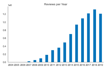The above figure shows the number of comments per year from 2004 to 2018
The above chart shows the average star rating of comments each year

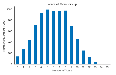
2. Visualization of member years details

#Draw a picture of the number of members each year
ax = yelp_reviews.member_yrs.value_counts().div(1000).sort_index().plot.bar(title='Years of Membership',
                                                                            rot=0)
ax.set_xlabel('Number of Years')
ax.set_ylabel("Number of Members  ('000)")
sns.despine()
plt.tight_layout()

3. Construct training set and test set

#Import data and build test sets and training sets
train = yelp_reviews[yelp_reviews.year < 2019].sample(frac=.25)
test = yelp_reviews[yelp_reviews.year == 2019]
train.to_parquet(text_features_dir / 'train.parquet')
test.to_parquet(text_features_dir / 'test.parquet')
del yelp_reviews
train = pd.read_parquet(text_features_dir / 'train.parquet')
test = pd.read_parquet(text_features_dir / 'test.parquet')#Reload stored data

4. Build a document for Yelp comments - term matrix

vectorizer = CountVectorizer(stop_words='english', ngram_range=(1, 2), max_features=10000)
train_dtm = vectorizer.fit_transform(train.text)
train_dtm
sparse.save_npz(text_features_dir / 'train_dtm', train_dtm)
test_dtm = vectorizer.transform(test.text)
sparse.save_npz(text_features_dir / 'test_dtm', test_dtm)

4. Combine digital features with document term matrix

The data set contains various digital features, and the vector generator generates SciPy Sparse matrix. In order to combine the vectorized text data with other features, these data must also be transformed into sparse matrix; Many sklearn objects and libraries, such as lightgbm, can handle these data structures. However, it should be noted that there is a risk of memory overflow when converting a sparse matrix to a dense numpy array.
Because most variables have categories, we use one hot encoding, and we have a fairly large data set that can adapt to the increase of features. Then combine the converted digital features with the document term matrix.

Single hot coding is one hot coding, also known as one bit effective coding. Its method is to use n-bit status registers to encode N states. Each state has its own register bits, and only one bit is effective at any time.

df = pd.concat([train.drop(['text', 'stars'], axis=1).assign(source='train'),
                test.drop(['text', 'stars'], axis=1).assign(source='test')])
uniques = df.nunique()
binned = pd.concat([(df.loc[:, uniques[uniques > 20].index]
                     .apply(pd.qcut, q=10, labels=False, duplicates='drop')),
                    df.loc[:, uniques[uniques <= 20].index]], axis=1)
binned.info(null_counts=True)
dummies = pd.get_dummies(binned, 
                         columns=binned.columns.drop('source'), 
                         drop_first=True)
dummies.info()   
train_dummies = dummies[dummies.source=='train'].drop('source', axis=1)
train_dummies.info()        

5. Datum accuracy
A benchmark accuracy is obtained by predicting the most frequent comment stars

#This code obtains a benchmark accuracy, that is, all use the five-star comments with the highest frequency to complete the prediction
accuracy, runtime = {}, {}
predictions = test[['stars']].copy()
naive_prediction = np.full_like(predictions.stars,
fill_value=train.stars.mode().iloc[0])
naive_benchmark = accuracy_score(predictions.stars, naive_prediction)
naive_benchmark

0.5117779042568241

The author believes that it is quite amazing that more than 50% of the prediction accuracy can be obtained by using such a simple prediction rule.

6. Multiclass naive Bayes
Next, a naive Bayesian classifier is trained using the document term matrix generated by countvector under the default setting.

nb = MultinomialNB()
result = 'nb_text'
evaluate_model(nb, train_dtm, test_dtm, result, store=False)

The accuracy of naive Bayes is tested

accuracy[result]

0.6520747864021135

The prediction obtained by naive Bayes has an accuracy of 64.4% on the test set, which is 24.2% higher than the benchmark value.

Confusion matrix
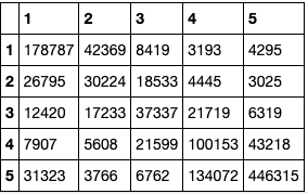The diagonal of the confusion matrix is the correct comment. The first row and the second column should be one star evaluation, but 42369 are predicted to be two star evaluation.
Next, the prediction accuracy after the combination of text and digital features is detected.

#The code segment can get the accuracy of the prediction method after the combination of text and digital features
result = 'nb_combined'
evaluate_model(nb, train_dtm_numeric, test_dtm_numeric, result, store=False)
accuracy[result]

0.6739017433272251

The combined accuracy is improved to 67%

7. Comparison between different models

#This code compares the performance of naive Bayes, logistic regression and LightGBM, and visualizes the results.
model_map = {'nb_combined': 'Naive Bayes',
             'lr_comb': 'Logistic Regression',
             'lgb_comb': 'LightGBM'}
accuracy_ = {model_map[k]: v for k, v in accuracy.items() if model_map.get(k)}
log_reg_text = pd.read_csv(yelp_dir / 'logreg_text.csv',
                       index_col=0,
                       squeeze=True)
log_reg_combined = pd.read_csv(yelp_dir / 'logreg_combined.csv',
                       index_col=0,
                       squeeze=True)
 log_reg_text = pd.read_csv(yelp_dir / 'logreg_text.csv',
                       index_col=0,
                       squeeze=True)
log_reg_combined = pd.read_csv(yelp_dir / 'logreg_combined.csv',
                       index_col=0,
                       squeeze=True)                      

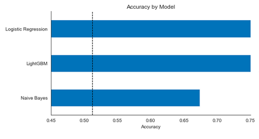As shown in the figure, logistic regression performs best, and the test accuracy is slightly higher than 74%, while naive Bayes performs worst among the three. But in fact, if we adjust the super parameters of the gradient enhancement model, the probability can increase its prediction accuracy, so that it can at least reach the level of logical regression.