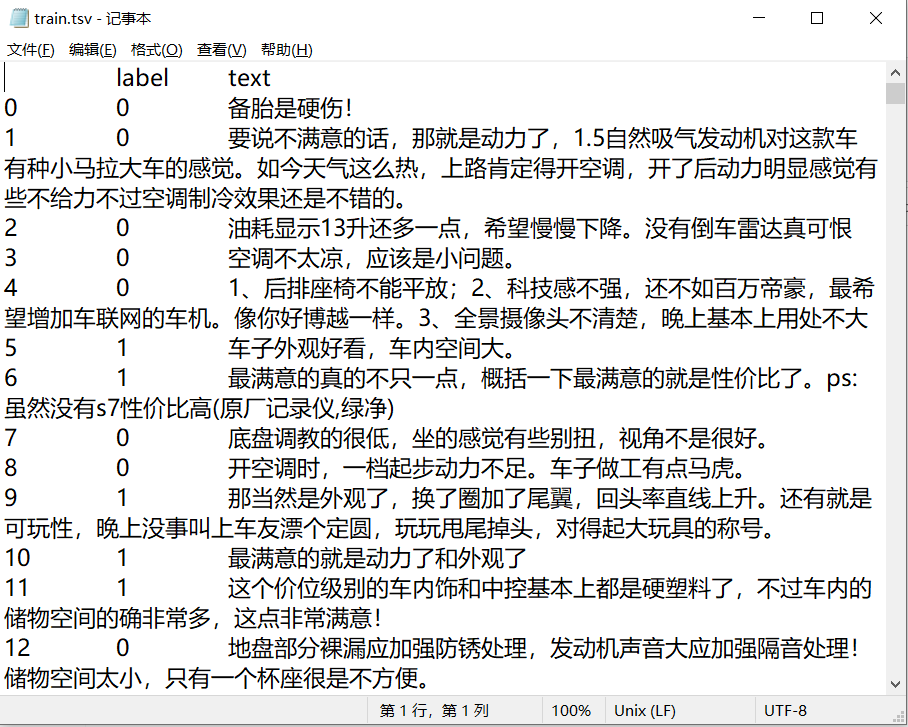
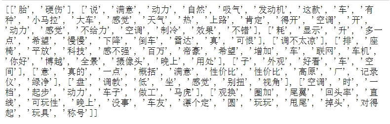
Recently, I learned the MLP, CNN and RNN network models based on pytoch framework, and conducted text classification experiments using the commodity comment data obtained on GitHub. This paper introduces how to establish MLP under the pytoch framework to classify the data. The data sets are roughly as follows:

1. Import module

import pandas as pd
import numpy as np
import jieba
import keras
import re
import spacy
from keras.preprocessing.text import Tokenizer
import gensim
from gensim import models
from torch.nn.utils.rnn import pad_sequence
import torch

2. Import data

data = pd.read_csv('./data.tsv',sep='\t',index_col=0).astype(str)
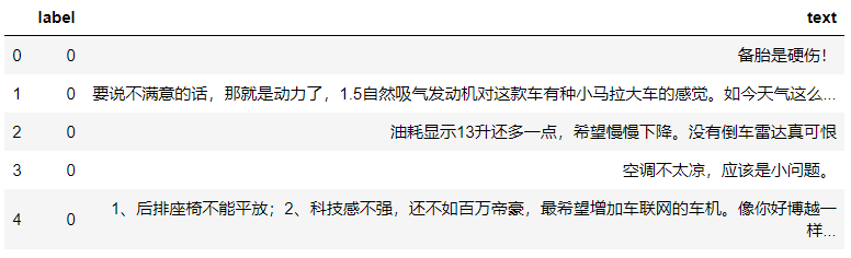
data.head()

3. Text data preprocessing

3.1 data cleaning

First of all, the data set needs to be cleaned routinely. In the actual e-commerce platform, sometimes users do not comment after purchase, and businesses automatically release high praise for the product in order to "brush the bill", so it is necessary to check the missing value, double value and delete the text data respectively, so as to reduce the unnecessary impact on the research purpose. At the same time, because too short comments are of little research value, the data with comment text less than or equal to 5 is filtered out. The above cleaning process is uniformly customized and packaged into the clean function as follows:

def clean(data):
    #Remove missing values
    Nan = data.dropna()
    print("After removing missing values:",Nan.shape)
    #Remove duplicate values
    dup = Nan.drop_duplicates()
    print("After removing duplicate values:",dup.shape)
    #Filter comments with more than 5 comment text
    clean_data = dup[dup['text'].str.len() > 5]
    print("After filtering out comments with more than 5 comment texts:",clean_data.shape)
    clean_data.reset_index(inplace=True)
    
    return clean_data

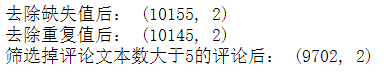
After running, it is found that there are no missing values in the data, but there are 10 duplicate values. After deleting the text data less than or equal to 5, 9702 comments remain.

3.2 word segmentation and removal of stop words

First, we need to exclude the text that is not Chinese characters, such as numbers and letters, and use the re module to define find_ The Chinese function is as follows:

#Exclude numbers, letters and other data that are not Chinese characters
def find_chinese(file):
    pattern = re.compile(r'[^\u4e00-\u9fa5]')
    chinese = re.sub(pattern, '', file)
    return chinese

for number in range(len(newdata)):
    newdata[number]=find_chinese(newdata[number])

Then use the jieba module to segment the text and store the results in the list, transfer in the xlsx file containing Chinese stop words data, and use the if judgment statement to remove the stop words (much faster than spacy...). These two steps can be packaged into the following functions:

#Remove stop words
def del_stop(texts):
    stop_words=pd.read_excel("stop_words.xlsx",header=None)[0].tolist()
    texts = list(map(find_chinese,texts))

    texts_temp = []
    n = 0

    for sentence in texts:
        n += 1
        doc = ''
        sentence_list = jieba.lcut(sentence)
        for word in sentence_list:
            if word not in stop_words:
                doc += word
        texts_temp.append(doc[1:])

    return texts_temp

#participle
def split_words(texts):
    texts_temp=[]

    for sentence in texts:

        sentence_list=jieba.lcut(sentence)
        texts_temp.append(" ".join(sentence_list))

    return texts_temp

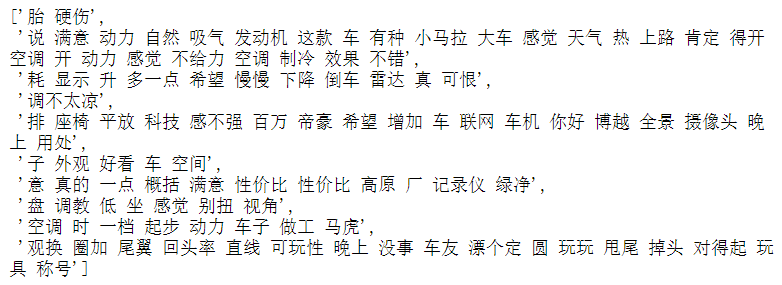
Print out the top ten items of the result list, as shown in the following figure:

3.3 text Vectorization

Because the ultimate purpose of the experiment is to classify the text, it is necessary to convert the text into a mathematical representation - vector, that is, word embedding technology. In this paper, Doc2Vec method is used to encapsulate each word in the text into vector expression, and Doc2Vec function in gensim module is used for training. According to the requirements of input parameters of this function, the data processed above needs to be converted again:

words = []

for i in result:
    a = i.split(' ')
    words.append(a)
    
print(words[:10])

It looks like this:

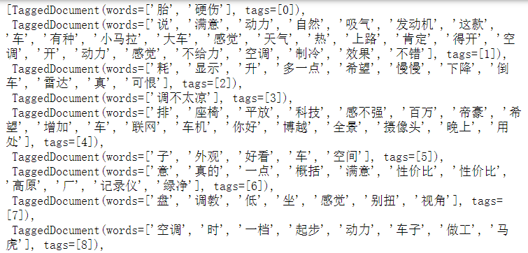
Then you need to tag the data with the TaggedDocument function:

from gensim.models.doc2vec import Doc2Vec, TaggedDocument
train_docs = []
for i, text in enumerate(words):
    document = TaggedDocument(text, tags=[i])
    train_docs.append(document)

After typing, see the following figure:

After the tag, you can throw it into the function for training ~ this paper sets the vector dimension vector_ The size is 50, the number of threads in the training model is 4, and the number of training iterations epochs is 5:

model_dm = Doc2Vec(train_docs, dm=1, min_count=1, window=3, vector_size=50, sample=1e-3, negative=5, workers=4)
model_dm.train(train_docs, total_examples=model_dm.corpus_count, epochs=5)

Because the training output result only vectorizes each word in the text data, it is necessary to combine the original label value and pass it into the MLP model for training:

doc_vec = []

for i in range(len(train_docs)):
    doc_vec.append(model_dm.dv[i].tolist())

data = pd.DataFrame(doc_vec)
newdata = pd.concat([data,label],axis=1)
newdata.head(3)

newdata.to_csv('doc2vec.txt',sep = '\t',header = False)

After vectorization, the length is as follows:

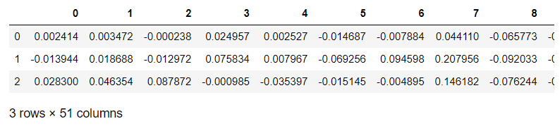
The merged data shape is 9702 rows and 51 columns (the last column is label), and the results are saved to the local txt file.

4. Build and train models

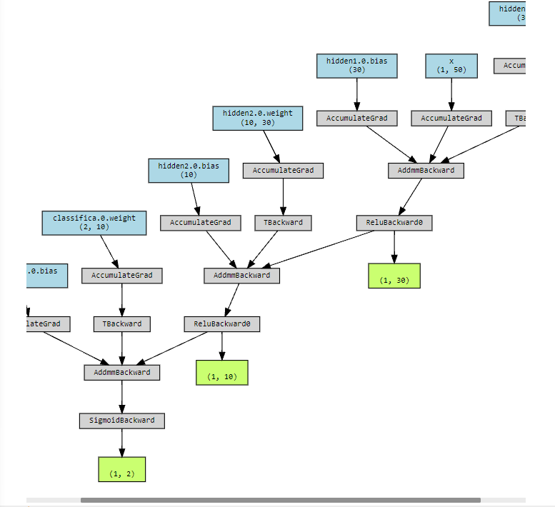
4.1 building MLP network

This part refers to the codes of books and teachers. Specifically, the MLP has two hidden layers, one classification layer, and defines the forward propagation path (the specific details will not be explained):

import torch.nn as nn

import torch
import matplotlib.pyplot as plt
from torchviz import make_dot
class MLPclassifica(nn.Module):
    def __init__(self):
        super(MLPclassifica,self).__init__()   ###Methods that inherit the parent class https://blog.csdn.net/a__int__/article/details/104600972 understanding of parent class inheritance
        #####Define the first hidden layer
        self.hidden1 = nn.Sequential(
            nn.Linear(
              in_features = 50,   ####Enter the number of features
              out_features = 30,  ####Number of output features
              bias = True,  ###bias
          ),
            nn.ReLU()
        )
        #####Define the second hidden as
        self.hidden2 = nn.Sequential(
            nn.Linear(30,10),
            nn.ReLU()
        )
        ######Classification layer
        self.classifica = nn.Sequential(
            nn.Linear(10,2),
            nn.Sigmoid()
        )
    #####Define forward propagation path
    def forward(self, x):
        fc1 = self.hidden1(x)
        fc2 = self.hidden2(fc1)
        output = self.classifica(fc2)
        ###The output is two hidden layers and an output layer
        return fc1,fc2,output

mlpc = MLPclassifica()
##visualization
x = torch.randn(1,50,requires_grad = True)
y = mlpc(x)
Mymlpcvis = make_dot(y, params=dict(list(mlpc.named_parameters())+ [('x',x)]))
Mymlpcvis

The network can be visualized as follows (seemingly incomplete):

4.2 training model

First, import relevant modules and cut the data into training set and test set:

import numpy as np
import pandas as pd
from sklearn.preprocessing import StandardScaler,MinMaxScaler
from sklearn.model_selection import train_test_split
from sklearn.metrics import accuracy_score,confusion_matrix,classification_report
from sklearn.manifold import TSNE


X_train, X_test, y_train, y_test = train_test_split(np.array(newdata.iloc[:,:50]),
                                                    np.array(newdata.iloc[:,50]),test_size=0.25, random_state=123)

Then, the training data and test data shall be converted into tensors respectively. After conversion, X and y shall be combined, and a data loader shall be defined to process the data in batch:

import torch.utils.data as Data

X_train_t = torch.from_numpy(X_train.astype(np.float32))
y_train_t = torch.from_numpy(y_train.astype(np.int64))
X_test_t = torch.from_numpy(X_test.astype(np.float32))
y_test_t = torch.from_numpy(y_test.astype(np.int64))

train_data = Data.TensorDataset(X_train_t,y_train_t)

train_loader = Data.DataLoader(
    dataset = train_data ,
    batch_size = 64 ,
    shuffle = True, ###Scramble data before each iteration
    num_workers = 3,   ##The number of processes loaded using multiple processes. 0 means that multiple processes are not used
)

Then you need to define an optimizer and visualize the results using Canvas. Finally, start training the model and set the number of training iterations epoch to 15:

###Load data to improve the whole network
from torch.optim import SGD,Adam
import seaborn as sns
import hiddenlayer as hl

###Define optimizer
optimizer = torch.optim.Adam(mlpc.parameters(),lr=0.01)
loss_func = nn.CrossEntropyLoss()    ###Binary loss function

####Record the indicators of the training process
history1 = hl.History()

####Visualization using Canvas
canvas1 = hl.Canvas()
print_step = 25

###Iterative training is carried out for the model, and epoch round is trained for all data
for epoch in range(15):
    ##Iterative calculation of the loader of training data
    for step, (b_x , b_y) in enumerate(train_loader):
        ##Calculate the loss per batch
        _, _, output = mlpc(b_x)   ###MLP output on training batch
        train_loss = loss_func(output , b_y)   ####Binary cross entropy loss function
        optimizer.zero_grad()     #####The gradient of each iteration is initialized to 0
        train_loss.backward()     #####The loss is propagated backward and the gradient is calculated
        optimizer.step()         #####Optimization using gradients
        niter = epoch*len(train_loader) + step +1
        if niter % print_step == 0:
            _, _, output = mlpc(X_test_t)
            _, pre_lab = torch.max(output, 1)
            test_accuracy = accuracy_score(y_test_t, pre_lab)
            ## Add epoch, loss, and precision to history
            history1.log(niter, train_loss=train_loss, test_accuracy=test_accuracy)
            ###Two images are used to visualize the loss function and accuracy
            with canvas1:
                canvas1.draw_plot(history1['train_loss'])
                canvas1.draw_plot(history1['test_accuracy'])

The results are as follows:

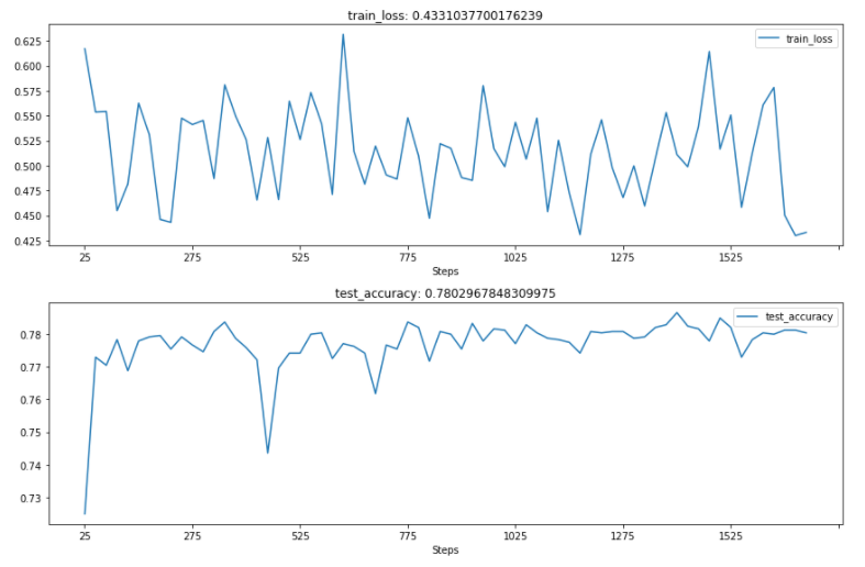
It can be seen that the accuracy of the test set is about 0.78.

5. Improvement direction

1. In this paper, the fixed stopwords data file is used to remove the stop words, and the influence of subject words on the results is not considered for the text data of different topics
2. To improve the accuracy of the model, we can refer to improving the vector dimension, training epoch times and so on