This article is shared from Huawei cloud community< Text classification based on Keras+RNN vs text classification based on traditional machine learning >, by eastmount.
1, RNN text classification
1.RNN
Cyclic neural networks is called Recurrent Neural Networks (RNN) in English. The essential concept of RNN is to use timing information. In traditional neural networks, it is assumed that all inputs (and outputs) are independent. However, for many tasks, this is very limited. For example, if you want to predict the next word based on an unfinished sentence, the best way is to contact the contextual information. The reason why RNN (cyclic neural network) is "cyclic" is that they perform the same task on each element of the sequence, and each result is independent of the previous calculation.
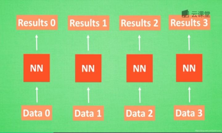
Suppose there is a set of data data0, data1, data2 and data3. Use the same neural network to predict them and get the corresponding results. If there is a relationship between the data, such as the steps before and after cooking and cutting, and the order of English words, how can the correlation between the data be learned by neural network? This requires RNN.
For example, if there is an ABCD number and the next number E needs to be predicted, it will be predicted according to the previous ABCD order, which is called memory. Before prediction, it is necessary to review the previous memory, plus the new memory points in this step, and finally output. This principle is used by recurrent neural network (RNN).
First, let's think about how humans analyze the relationship or order between things. Humans usually remember what happened before, so as to help us judge our subsequent behavior. Can computers also remember what happened before?
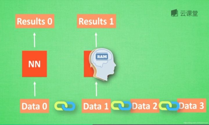
When analyzing data0, we store the analysis results in Memory memory. Then when analyzing data1, neural network (NN) will generate new Memory, but the new Memory is not associated with the old Memory, as shown in the above figure. In RNN, we will simply call the old Memory to analyze the new Memory. If we continue to analyze more data, NN will accumulate all the previous memories.
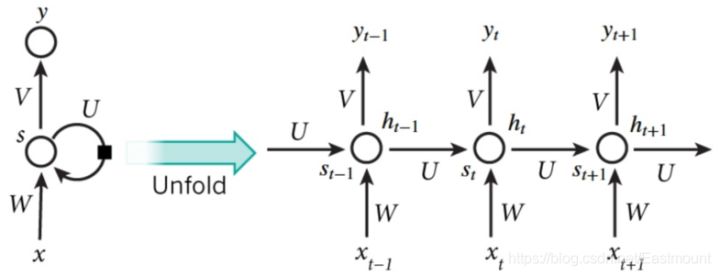
The following is a typical RNN result model. According to the time points t-1, t and t+1, there are different x at each time. Each calculation will consider the state of the previous step and x(t) of this step, and then output the y value. In this mathematical form, s(t) will be generated after each RNN run. When RNN wants to analyze x(t+1), y(t+1) at the moment is jointly created by s(t) and s(t+1), and s(t) can be regarded as the memory of the previous step. The accumulation of multiple neural networks NN is converted into a cyclic neural network, and its simplified diagram is shown on the left of the figure below. For example, if the sentence in the sequence has five words, then there will be five layers of neural network after expanding the network horizontally, one layer corresponds to one word.
In short, as long as your data is in order, you can use RNN, such as the order of human speech, the order of telephone numbers, the order of image pixels, the order of ABC letters, etc. RNN is commonly used in natural language processing, machine translation, speech recognition, image recognition and other fields.
2. Text classification
Text classification aims to automatically classify and mark the text set according to a certain classification system or standard. It belongs to an automatic classification based on the classification system. Text classification can be traced back to the 1950s, when text classification was mainly carried out through expert defined rules; In the 1980s, the expert system established by knowledge engineering appeared; In the 1990s, text classification was carried out through artificial feature engineering and shallow classification model with the help of machine learning method. At present, word vector and deep neural network are mostly used for text classification.
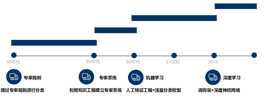
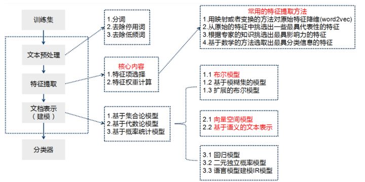
Teacher Niu Yafeng summarized the traditional text classification process as shown in the figure below. In the traditional text classification, most machine learning methods are basically applied in the field of text classification. It mainly includes:
- Naive Bayes
- KNN
- SVM
- Collection class method
- Maximum entropy
- neural network
The basic process of text classification using Keras framework is as follows:
- Step 1: text preprocessing, word segmentation - > remove stop words - > statistics, select top n words as feature words
- Step 2: generate ID for each feature word
- Step 3: convert the text into ID sequence and fill the left
- Step 4: training set shuffle
- Step 5: Embedding Layer converts words into word vectors
- Step 6: add the model and construct the neural network structure
- Step 7: Training Model
- Step 8: get the accuracy, recall and F1 value
Note that if TFIDF is used instead of word vector for document representation, the TFIDF matrix is generated after word segmentation and stop, and then the model is input. This paper will use word vector and TFIDF to experiment.
Deep learning text classification methods include:
- Convolutional neural network (TextCNN)
- Cyclic neural network (TextRNN)
- TextRNN+Attention
- TextRCNN(TextRNN+CNN)
Recommended articles by Niu Yafeng: Text Classification Based on word2vec and CNN: Review & Practice
2, Text classification based on traditional machine learning Bayesian algorithm
1.MultinomialNB+TFIDF text classification
The data set adopts Mr. Ji Jiwei's user-defined text, with a total of 21 lines of data, including 2 categories (Xiaomi mobile phone and Xiaomi porridge). The basic process is:
- Get dataset data and target
- Call Jieba library to realize Chinese word segmentation
- Calculate the TF-IDF value and convert the word frequency matrix into TF-IDF vector matrix
- Call machine learning algorithm for training and prediction
- Experimental evaluation and visual analysis
The complete code is as follows:
# -*- coding: utf-8 -*-
"""
Created on Sat Mar 28 22:10:20 2020
@author: Eastmount CSDN
"""
from jieba import lcut
#--------------------------------Loading data and preprocessing-------------------------------
data = [
[0, 'Millet porridge is a kind of porridge made of millet as the main ingredient. It has light taste and fragrance. It is simple and easy to make, good for the stomach and digestion'],
[0, 'When cooking porridge, be sure to boil water first, and then put in the washed millet'],
[0, 'Protein and amino acids, fat, vitamins, minerals'],
[0, 'Millet is a traditional healthy food, which can be stewed and porridge alone'],
[0, 'Apple is a kind of fruit'],
[0, 'Porridge has high nutritional value, rich in minerals and vitamins, rich in calcium, which helps to metabolize the excess salt in the body'],
[0, 'Eggs have high nutritional value and are high-quality protein B A good source of vitamins, but also provide fat, vitamins and minerals'],
[0, 'The apples in this supermarket are very fresh'],
[0, 'In the north, millet is one of the main foods, and many areas have the custom of eating millet porridge for dinner'],
[0, 'Millet has high nutritional value, comprehensive and balanced nutrition, and mainly contains carbohydrates'],
[0, 'Protein, amino acid, fat, vitamin and salt'],
[1, 'Xiaomi, Samsung and Huawei are the three flagship mobile phones of Android'],
[1, 'Forget about Xiaomi Huawei! Meizu mobile phone re exposure: This is really perfect'],
[1, 'Apple may return to 2016, but this time it can't raise prices significantly'],
[1, 'Samsung wants to continue to suppress Huawei, just by A70 not enough yet'],
[1, 'Samsung's mobile screen will reach a new high, surpassing Huawei and Apple's flagship'],
[1, 'Huawei P30,Samsung A70 Sold like hot cakes and won Suning's best mobile phone marketing award'],
[1, 'Lei Jun, tell you with a picture: where is the gap between Xiaomi and Samsung'],
[1, 'Xiaomi chat APP official Linux Version on-line, adaptive depth system'],
[1, 'Samsung has just updated its wearable device APP'],
[1, 'The cross-border between Huawei and Xiaomi is not terrible. It can't break the inner "ceiling"'],
]
#Chinese analysis
X, Y = [' '.join(lcut(i[1])) for i in data], [i[0] for i in data]
print(X)
print(Y)
#['when cooking porridge, be sure to boil water first, and then put in the washed millet',...]
#--------------------------------------Calculate word frequency------------------------------------
from sklearn.feature_extraction.text import CountVectorizer
from sklearn.feature_extraction.text import TfidfTransformer
#Convert words in text into word frequency matrix
vectorizer = CountVectorizer()
#Count the number of occurrences of a word
X_data = vectorizer.fit_transform(X)
print(X_data)
#Get all text keywords in the word bag
word = vectorizer.get_feature_names()
print('[View words]')
for w in word:
print(w, end = " ")
else:
print("\n")
#frequency matrix
print(X_data.toarray())
#Count the word frequency matrix X into TF-IDF value
transformer = TfidfTransformer()
tfidf = transformer.fit_transform(X_data)
#The view data structure tfidf[i][j] represents the TF IDF weight in class I text
weight = tfidf.toarray()
print(weight)
#--------------------------------------Data analysis------------------------------------
from sklearn.naive_bayes import MultinomialNB
from sklearn.metrics import classification_report
from sklearn.model_selection import train_test_split
X_train, X_test, y_train, y_test = train_test_split(weight, Y)
print(len(X_train), len(X_test))
print(len(y_train), len(y_test))
print(X_train)
#Call MultinomialNB classifier
clf = MultinomialNB().fit(X_train, y_train)
pre = clf.predict(X_test)
print("Prediction results:", pre)
print("Real results:", y_test)
print(classification_report(y_test, pre))
#--------------------------------------Visual analysis------------------------------------
#Dimensionality reduction drawing
from sklearn.decomposition import PCA
import matplotlib.pyplot as plt
pca = PCA(n_components=2)
newData = pca.fit_transform(weight)
print(newData)
L1 = [n[0] for n in newData]
L2 = [n[1] for n in newData]
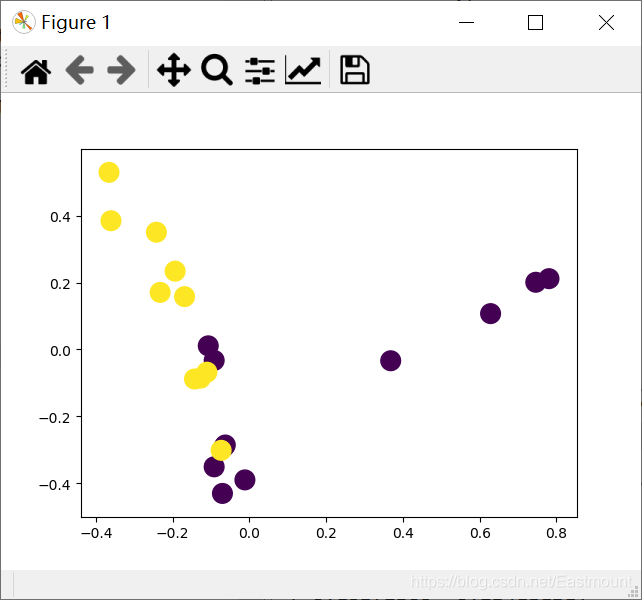
plt.scatter(L1, L2, c=Y, s=200)
plt.show()The output results are as follows:
- Accuracy of 6 forecast data = = > 0.67
['Millet porridge is a kind of porridge made of millet as the main ingredient. It has light taste and fragrance. It is simple and easy to make, good for the stomach and digestion',
 'When cooking porridge, be sure to boil water first, and then put in the washed millet',
 'Protein and amino acids, fat, vitamins, minerals',
 ...
 'Samsung has just updated its wearable device APP',
 'The cross-border between Huawei and Xiaomi is not terrible. It can't break the inner "ceiling"']
[0, 0, 0, 0, 0, 0, 0, 0, 0, 0, 0, 1, 1, 1, 1, 1, 1, 1, 1, 1, 1]

[View words]
2016 app linux p30 It must be a Samsung health card ... Lei Jun food ingredients Meizu eggs

[[0 0 0 ... 0 0 0]
 [0 0 0 ... 0 0 0]
 [0 0 0 ... 0 0 0]
 ...
 [0 0 1 ... 0 0 0]
 [0 0 1 ... 0 0 0]
 [0 0 0 ... 0 0 0]]

15 6
15 6
[[0.         0.         0.         ... 0.         0.         0.        ]
 [0.         0.         0.         ... 0.         0.         0.32161043]
 [0.         0.         0.         ... 0.         0.         0.        ]
 ...
 [0.         0.31077094 0.         ... 0.         0.         0.        ]
 [0.         0.         0.         ... 0.         0.         0.        ]
 [0.35882035 0.         0.         ... 0.         0.         0.        ]]
Prediction results: [0 1 0 1 1 1]
Real results: [0, 0, 0, 0, 1, 1]

              precision    recall  f1-score   support

           0       1.00      0.50      0.67         4
           1       0.50      1.00      0.67         2

    accuracy                           0.67         6
   macro avg       0.75      0.75      0.67         6
weighted avg       0.83      0.67      0.67         6
The drawing is shown in the following figure:
2. Gaussian Nb + word2vec text classification
The difference between this method and the previous method is that Word2Vec is used to calculate the word vector, divide each row of data set into words, calculate the word vector of each feature word, and then convert it into a word vector matrix, such as 15 rows of data, 40 feature words per row of data, and each feature word is represented by a word direction quantity of 20 dimensions, i.e. (15, 40, 20). At the same time, because the word vector has negative numbers, it is necessary to use Gaussian NB algorithm instead of MultinomialNB algorithm.
For details of Word2Vec, see the author's previous article: [Python artificial intelligence] IX. installation of gensim word vector Word2Vec and similarity calculation of Chinese short text of Qing Nian
- Senses: list of lists of tokens. The default value is None
- size: Dimension of word vector. The default value is 100
- window: the maximum distance between the current word and the predicted word in the same sentence. The default value is 5
- min_count: the minimum word frequency filter. The default value is 5
- workers: number of threads. The default value is 3
- sg: model parameter. A value of 0 indicates CBOW, a value of 1 indicates skip gram, and the default value is 0
- hs: model parameter. A value of 0 indicates negative sampling, a value of 1 indicates hierarchical softmax, and the default value is 0
- Negative: the number of negative samples. The default value is 5
- ns_exponent: the exponent used to form the negative sample. The default value is 0.75
- cbow_mean: context word vector parameter. A value of 0 indicates the summation value of context word vector. A value of 1 indicates the average value of context word vector. The default value is 1
- alpha: initial learning rate. The default value is 0.025
- min_alpha: minimum learning rate. The default value is 0.0001
The complete code is as follows:
# -*- coding: utf-8 -*-
"""
Created on Sat Mar 28 22:10:20 2020
@author: Eastmount CSDN
"""
from jieba import lcut
from numpy import zeros
from gensim.models import Word2Vec
from sklearn.model_selection import train_test_split
from tensorflow.python.keras.preprocessing.sequence import pad_sequences

max_features = 20                  #Word vector dimension
maxlen = 40                        #Maximum length of sequence

#--------------------------------Loading data and preprocessing-------------------------------
data = [
    [0, 'Millet porridge is a kind of porridge made of millet as the main ingredient. It has light taste and fragrance. It is simple and easy to make, good for the stomach and digestion'],
    [0, 'When cooking porridge, be sure to boil water first, and then put in the washed millet'],
    [0, 'Protein and amino acids, fat, vitamins, minerals'],
    [0, 'Millet is a traditional healthy food, which can be stewed and porridge alone'],
    [0, 'Apple is a kind of fruit'],
    [0, 'Porridge has high nutritional value, rich in minerals and vitamins, rich in calcium, which helps to metabolize the excess salt in the body'],
    [0, 'Eggs have high nutritional value and are high-quality protein B A good source of vitamins, but also provide fat, vitamins and minerals'],
    [0, 'The apples in this supermarket are very fresh'],
    [0, 'In the north, millet is one of the main foods, and many areas have the custom of eating millet porridge for dinner'],
    [0, 'Millet has high nutritional value, comprehensive and balanced nutrition, and mainly contains carbohydrates'],
    [0, 'Protein, amino acid, fat, vitamin and salt'],
    [1, 'Xiaomi, Samsung and Huawei are the three flagship mobile phones of Android'],
    [1, 'Forget about Xiaomi Huawei! Meizu mobile phone re exposure: This is really perfect'],
    [1, 'Apple may return to 2016, but this time it can't raise prices significantly'],
    [1, 'Samsung wants to continue to suppress Huawei, just by A70 not enough yet'],
    [1, 'Samsung's mobile screen will reach a new high, surpassing Huawei and Apple's flagship'],
    [1, 'Huawei P30,Samsung A70 Sold like hot cakes and won Suning's best mobile phone marketing award'],
    [1, 'Lei Jun, tell you with a picture: where is the gap between Xiaomi and Samsung'],
    [1, 'Xiaomi chat APP official Linux Version on-line, adaptive depth system'],
    [1, 'Samsung has just updated its wearable device APP'],
    [1, 'The cross-border between Huawei and Xiaomi is not terrible. It can't break the inner "ceiling"'],
]

#Chinese analysis
X, Y = [lcut(i[1]) for i in data], [i[0] for i in data]

#Partition training set and prediction set
X_train, X_test, y_train, y_test = train_test_split(X, Y)
#print(X_train)
print(len(X_train), len(X_test))
print(len(y_train), len(y_test))
"""['Samsung', 'just', 'to update', 'Yes', 'Own', 'of', 'can', 'wear', 'equipment', 'APP']"""

#--------------------------------Word2Vec word vector-------------------------------
word2vec = Word2Vec(X_train, size=max_features, min_count=1) #Maximum characteristic minimum filtering frequency 1
print(word2vec)

#Mapping feature words
w2i = {w:i for i, w in enumerate(word2vec.wv.index2word)}
print("[Show words]")
print(word2vec.wv.index2word)
print(w2i)
"""['millet', 'Samsung', 'yes', 'vitamin', 'protein', 'and', 'APP', 'amino acid',..."""
"""{',': 0, 'of': 1, 'millet': 2, ',': 3, 'Huawei': 4, ....}"""

#Word vector calculation
vectors = word2vec.wv.vectors
print("[Word vector matrix]")
print(vectors.shape)
print(vectors)

#Custom function - get word vector
def w2v(w):
    i = w2i.get(w)
    return vectors[i] if i else zeros(max_features)

#Custom function - sequence preprocessing
def pad(ls_of_words):
    a = [[w2v(i) for i in x] for x in ls_of_words]
    a = pad_sequences(a, maxlen, dtype='float')
    return a

#The serialization process is converted to a word vector
X_train, X_test = pad(X_train), pad(X_test)
print(X_train.shape)
print(X_test.shape)
"""(15, 40, 20) 15 A sample of 40 features, each feature is represented by a 20 word vector"""

#Straightening shape (15, 40, 20) = > (15, 40 * 20) (6, 40, 20) = > (6, 40 * 20)
X_train = X_train.reshape(len(y_train), maxlen*max_features)
X_test = X_test.reshape(len(y_test), maxlen*max_features)
print(X_train.shape)
print(X_test.shape)

#--------------------------------Modeling and training-------------------------------
from sklearn.naive_bayes import GaussianNB
from sklearn.metrics import classification_report
from sklearn.model_selection import train_test_split

#Call Gaussian NB classifier
clf = GaussianNB().fit(X_train, y_train)
pre = clf.predict(X_test)
print("Prediction results:", pre)
print("Real results:", y_test)
print(classification_report(y_test, pre))
The output results are as follows:
- Accuracy of 6 forecast data = = > 0.83
15 6
15 6
Word2Vec(vocab=126, size=20, alpha=0.025)

[Show words]
[',', ',', 'millet', 'of', 'Huawei', 'mobile phone', 'Apple', 'vitamin', 'APP', 'official', 'Linux', ... 'An Zhuo San Da', 'flagship']
{',': 0, ',': 1, 'millet': 2, 'of': 3, 'Huawei': 4, 'mobile phone': 5, 'Apple': 6,  ...,  'An Zhuo San Da': 124, 'flagship': 125}

[Word vector matrix]
(126, 20)
[[ 0.02041552 -0.00929706 -0.00743623 ... -0.00246041 -0.00825108
   0.02341811]
 [-0.00256093 -0.01301112 -0.00697959 ... -0.00449076 -0.00551124
  -0.00240511]
 [ 0.01535473  0.01690796 -0.00262145 ... -0.01624218  0.00871249
  -0.01159615]
 ...
 [ 0.00631155  0.00369085 -0.00382834 ...  0.02468265  0.00945442
  -0.0155745 ]
 [-0.01198495  0.01711261  0.01097644 ...  0.01003117  0.01074963
   0.01960118]
 [ 0.00450704 -0.01114052  0.0186879  ...  0.00804681  0.01060277
   0.01836049]]

(15, 40, 20)
(6, 40, 20)
(15, 800)
(6, 800)

Prediction results: [1 1 1 0 1 0]
Real results: [0, 1, 1, 0, 1, 0]
              precision    recall  f1-score   support

           0       1.00      0.67      0.80         3
           1       0.75      1.00      0.86         3

    accuracy                           0.83         6
   macro avg       0.88      0.83      0.83         6
weighted avg       0.88      0.83      0.83         6
3, Implementation of RNN text classification by Keras
1.IMDB dataset and sequence preprocessing
(1) IMDB dataset
The Keras framework provides us with some commonly used built-in data sets. For example, handwriting recognition MNIST data set in the field of image recognition, film review imdb data set in the field of text classification, and so on. These databases can be called with one code:
- (trainX, trainY), (testX, testY) = imdb.load_data(path="imdb.npz", num_words=max_features)
These data sets are through https://s3.amazonaws.com Download, but sometimes the website cannot be used. You need to download data locally and then call for analysis. Keras dataset Baidu cloud link:
- https://pan.baidu.com/s/1aZRp0uMkNj2QEWYstaNsKQ , extraction code: 3a2u
The author puts the downloaded data in the C:\Users\Administrator.keras\datasets folder, as shown in the following figure.
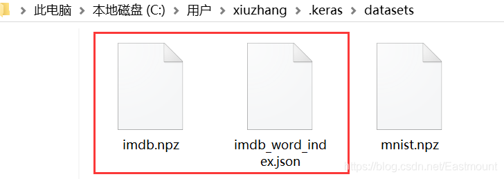
This data set is the Internet Movie Database (IMDb), which is an online database about movie actors, movies, TV programs, TV stars and movie production.
The data and format in imdb.npz file are as follows:
[list([1, 14, 22, 16, 43, 530, 973, 1622, 1385, 65, 458, 4468, 66, 3941, 4, 173, 36, 256, 5, 25, 100, 43, 838, 112, 50, 670, 2, 9, 35, 480, 284, 5, 150, 4, 172, ...])
 list([1, 194, 1153, 194, 8255, 78, 228, 5, 6, 1463, 4369, 5012, 134, 26, 4, 715, 8, 118, 1634, 14, 394, 20, 13, 119, 954, 189, 102, 5, 207, 110, 3103, 21, 14, 69, ...])
 list([1, 14, 47, 8, 30, 31, 7, 4, 249, 108, 7, 4, 5974, 54, 61, 369, 13, 71, 149, 14, 22, 112, 4, 2401, 311, 12, 16, 3711, 33, 75, 43, 1829, 296, 4, 86, 320, 35, ...])
 ...
 list([1, 11, 6, 230, 245, 6401, 9, 6, 1225, 446, 2, 45, 2174, 84, 8322, 4007, 21, 4, 912, 84, 14532, 325, 725, 134, 15271, 1715, 84, 5, 36, 28, 57, 1099, 21, 8, 140, ...])
 list([1, 1446, 7079, 69, 72, 3305, 13, 610, 930, 8, 12, 582, 23, 5, 16, 484, 685, 54, 349, 11, 4120, 2959, 45, 58, 1466, 13, 197, 12, 16, 43, 23, 2, 5, 62, 30, 145, ...])
 list([1, 17, 6, 194, 337, 7, 4, 204, 22, 45, 254, 8, 106, 14, 123, 4, 12815, 270, 14437, 5, 16923, 12255, 732, 2098, 101, 405, 39, 14, 1034, 4, 1310, 9, 115, 50, 305, ...])] train sequences
Each list is a sentence, and each number in the sentence represents the number of words. So, how to get the word corresponding to the number? You need to use IMDB at this time_ word_ Index.json file, the file format is as follows:
{"fawn": 34701, "tsukino": 52006,..., "paget": 18509, "expands": 20597}There are 88584 words in total, which are stored in key value format. Key represents word and value represents (word) number. The higher the word frequency (the number of words in the corpus), the smaller the number. For example, "the:1" has the highest number, and the number is 1.
(2) Sequence preprocessing
Pad is usually used in the process of deep learning vector conversion_ Sequences() sequence filling. Its basic usage is as follows:
keras.preprocessing.sequence.pad_sequences(
    sequences,
	maxlen=None,
	dtype='int32',
	padding='pre',
	truncating='pre',
	value=0.
	)
The parameters have the following meanings:
- sequences: a two-level nested list of floating-point numbers or integers
- maxlen: None or integer, which is the maximum length of the sequence. Sequences greater than this length will be truncated, and sequences less than this length will be filled with 0 at the back
- dtype: the data type of the returned numpy array
- padding: pre or post, which determines whether to supplement 0 at the beginning or end of the sequence when it is necessary to supplement 0
- truncating: pre or post, which determines whether to truncate the sequence from the beginning or the end when it is necessary to truncate the sequence
- Value: floating point number. This value will replace the default padding value of 0 during padding
- The return value is a 2-dimensional tensor with a length of maxlen
The basic usage is as follows:
from keras.preprocessing.sequence import pad_sequences

print(pad_sequences([[1, 2, 3], [1]], maxlen=2))
"""[[2 3] [0 1]]"""
print(pad_sequences([[1, 2, 3], [1]], maxlen=3, value=9))
"""[[1 2 3] [9 9 1]]"""

print(pad_sequences([[2,3,4]], maxlen=10))
"""[[0 0 0 0 0 0 0 2 3 4]]"""
print(pad_sequences([[1,2,3,4,5],[6,7]], maxlen=10))
"""[[0 0 0 0 0 1 2 3 4 5] [0 0 0 0 0 0 0 0 6 7]]"""

print(pad_sequences([[1, 2, 3], [1]], maxlen=2, padding='post'))
"""End position supplement: [[2 3] [1 0]]"""
print(pad_sequences([[1, 2, 3], [1]], maxlen=4, truncating='post'))
"""Start position supplement: [[0 1 2 3] [0 0 0 1]]"""
In natural language, it is generally used with word segmentation.
>>> tokenizer.texts_to_sequences(["I work overtime when it rains"])
[[4, 5, 6, 7]]

>>> keras.preprocessing.sequence.pad_sequences(tokenizer.texts_to_sequences(["I work overtime when it rains"]), maxlen=20)
array([[0, 0, 0, 0, 0, 0, 0, 0, 0, 0, 0, 0, 0, 0, 0, 0, 4, 5, 6, 7]],dtype=int32)
2. Word embedding model training
At this time, we will train through the word embedding model. The specific process includes:
- Import IMDB dataset
- Convert dataset to sequence
- Create Embedding word Embedding model
- Neural network training
The complete code is as follows:
# -*- coding: utf-8 -*-
"""
Created on Sat Mar 28 17:08:28 2020
@author: Eastmount CSDN
"""
from keras.datasets import imdb #Movie Database
from keras.preprocessing import sequence
from keras.models import Sequential
from keras.layers import Dense, Flatten, Embedding
#-----------------------------------Define parameters-----------------------------------
max_features = 20000 #Take the first 20000 words of the sample according to the word frequency
input_dim = max_features #Thesaurus size must be > = max_ features
maxlen = 80 #Maximum sentence length
batch_size = 128 #batch quantity
output_dim = 40 #Word vector dimension
epochs = 2 #Training batch
#--------------------------------Loading data and preprocessing-------------------------------
#Data acquisition
(trainX, trainY), (testX, testY) = imdb.load_data(path="imdb.npz", num_words=max_features)
print(trainX.shape, trainY.shape) #(25000,) (25000,)
print(testX.shape, testY.shape) #(25000,) (25000,)
#The sequence is truncated or supplemented to equal length
trainX = sequence.pad_sequences(trainX, maxlen=maxlen)
testX = sequence.pad_sequences(testX, maxlen=maxlen)
print('trainX shape:', trainX.shape)
print('testX shape:', testX.shape)
#------------------------------------Create model------------------------------------
model = Sequential()
#Word embedding: thesaurus size, word vector dimension, fixed sequence length
model.add(Embedding(input_dim, output_dim, input_length=maxlen))
#Flattening: maxlen*output_dim
model.add(Flatten())
#Output layer: 2 classification
model.add(Dense(units=1, activation='sigmoid'))
#Binary cross entropy loss of RMSprop optimizer
model.compile('rmsprop', 'binary_crossentropy', ['acc'])
#train
model.fit(trainX, trainY, batch_size, epochs)
#Model visualization
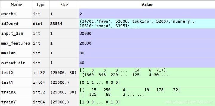
model.summary()The output results are as follows:
(25000,) (25000,)
(25000,) (25000,)
trainX shape: (25000, 80)
testX shape: (25000, 80)

Epoch 1/2
25000/25000 [==============================] - 2s 98us/step - loss: 0.6111 - acc: 0.6956
Epoch 2/2
25000/25000 [==============================] - 2s 69us/step - loss: 0.3578 - acc: 0.8549
Model: "sequential_2"
_________________________________________________________________
Layer (type)                 Output Shape              Param #
=================================================================
embedding_2 (Embedding)      (None, 80, 40)            800000
_________________________________________________________________
flatten_2 (Flatten)          (None, 3200)              0
_________________________________________________________________
dense_2 (Dense)              (None, 1)                 3201
=================================================================
Total params: 803,201
Trainable params: 803,201
Non-trainable params: 0
_________________________________________________________________
The display matrix is shown in the following figure:
3.RNN text classification
The complete code for text classification of IMDB movie dataset by RNN is as follows:
# -*- coding: utf-8 -*-
"""
Created on Sat Mar 28 17:08:28 2020
@author: Eastmount CSDN
"""
from keras.datasets import imdb  #Movie Database
from keras.preprocessing import sequence
from keras.models import Sequential
from keras.layers import Dense, Flatten, Embedding
from keras.layers import SimpleRNN

#-----------------------------------Define parameters-----------------------------------
max_features = 20000       #Take the first 20000 words of the sample according to the word frequency
input_dim = max_features   #Thesaurus size must be > = max_ features
maxlen = 40                #Maximum sentence length
batch_size = 128           #batch quantity
output_dim = 40            #Word vector dimension
epochs = 3                 #Training batch
units = 32                 #Number of RNN neurons

#--------------------------------Loading data and preprocessing-------------------------------
#Data acquisition
(trainX, trainY), (testX, testY) = imdb.load_data(path="imdb.npz", num_words=max_features)
print(trainX.shape, trainY.shape)  #(25000,) (25000,)
print(testX.shape, testY.shape)    #(25000,) (25000,)

#The sequence is truncated or supplemented to equal length
trainX = sequence.pad_sequences(trainX, maxlen=maxlen)
testX = sequence.pad_sequences(testX, maxlen=maxlen)
print('trainX shape:', trainX.shape)
print('testX shape:', testX.shape)

#-----------------------------------Create RNN model-----------------------------------
model = Sequential()

#Word embedding thesaurus size, word vector dimension, fixed sequence length
model.add(Embedding(input_dim, output_dim, input_length=maxlen))

#RNN Cell
model.add(SimpleRNN(units, return_sequences=True))   #Returns all results of the sequence
model.add(SimpleRNN(units, return_sequences=False))  #Returns the last result of the sequence

#Output layer 2 classification
model.add(Dense(units=1, activation='sigmoid'))

#Model visualization
model.summary()

#-----------------------------------Modeling and training-----------------------------------
#Activating neural network
model.compile(optimizer = 'rmsprop',              #RMSprop optimizer
              loss = 'binary_crossentropy',       #Binary cross entropy loss
              metrics = ['accuracy']              #Calculation error or accuracy
              )

#train
history = model.fit(trainX,
                    trainY,
                    batch_size=batch_size,
                    epochs=epochs,
                    verbose=2,
                    validation_split=.1            #Take 10% samples for verification
                    )

#-----------------------------------Prediction and visualization-----------------------------------
import matplotlib.pyplot as plt
accuracy = history.history['accuracy']
val_accuracy = history.history['val_accuracy']
plt.plot(range(epochs), accuracy)
plt.plot(range(epochs), val_accuracy)
plt.show()
The output results are as follows, three Epoch training.
- Accuracy of training data = = > 0.9075
- Value of evaluation data_ accuracy ===> 0.7844
Epoch can be represented vividly in the figure below.
(25000,) (25000,)
(25000,) (25000,)
trainX shape: (25000, 40)
testX shape: (25000, 40)
Model: "sequential_2"
_________________________________________________________________
Layer (type)                 Output Shape              Param #
=================================================================
embedding_2 (Embedding)      (None, 40, 40)            800000
_________________________________________________________________
simple_rnn_3 (SimpleRNN)     (None, 40, 32)            2336
_________________________________________________________________
simple_rnn_4 (SimpleRNN)     (None, 32)                2080
_________________________________________________________________
dense_2 (Dense)              (None, 1)                 33
=================================================================
Total params: 804,449
Trainable params: 804,449
Non-trainable params: 0
_________________________________________________________________

Train on 22500 samples, validate on 2500 samples
Epoch 1/3
 - 11s - loss: 0.5741 - accuracy: 0.6735 - val_loss: 0.4462 - val_accuracy: 0.7876
Epoch 2/3
 - 14s - loss: 0.3572 - accuracy: 0.8430 - val_loss: 0.4928 - val_accuracy: 0.7616
Epoch 3/3
 - 12s - loss: 0.2329 - accuracy: 0.9075 - val_loss: 0.5050 - val_accuracy: 0.7844
Accuracy and val drawn_ The accuracy curve is shown in the following figure:
- loss: 0.2329 - accuracy: 0.9075 - val_loss: 0.5050 - val_accuracy: 0.7844

4, RNN realizes text classification of Chinese data sets
1.RNN+Word2Vector text classification
The first step is to import the text dataset and convert it into a word vector.
data = [
    [0, 'Millet porridge is a kind of porridge made of millet as the main ingredient. It has light taste and fragrance. It is simple and easy to make, good for the stomach and digestion'],
    [0, 'When cooking porridge, be sure to boil water first, and then put in the washed millet'],
    [0, 'Protein and amino acids, fat, vitamins, minerals'],
    [0, 'Millet is a traditional healthy food, which can be stewed and porridge alone'],
    [0, 'Apple is a kind of fruit'],
    [0, 'Porridge has high nutritional value, rich in minerals and vitamins, rich in calcium, which helps to metabolize the excess salt in the body'],
    [0, 'Eggs have high nutritional value and are high-quality protein B A good source of vitamins, but also provide fat, vitamins and minerals'],
    [0, 'The apples in this supermarket are very fresh'],
    [0, 'In the north, millet is one of the main foods, and many areas have the custom of eating millet porridge for dinner'],
    [0, 'Millet has high nutritional value, comprehensive and balanced nutrition, and mainly contains carbohydrates'],
    [0, 'Protein, amino acid, fat, vitamin and salt'],
    [1, 'Xiaomi, Samsung and Huawei are the three flagship mobile phones of Android'],
    [1, 'Forget about Xiaomi Huawei! Meizu mobile phone re exposure: This is really perfect'],
    [1, 'Apple may return to 2016, but this time it can't raise prices significantly'],
    [1, 'Samsung wants to continue to suppress Huawei, just by A70 not enough yet'],
    [1, 'Samsung's mobile screen will reach a new high, surpassing Huawei and Apple's flagship'],
    [1, 'Huawei P30,Samsung A70 Sold like hot cakes and won Suning's best mobile phone marketing award'],
    [1, 'Lei Jun, tell you with a picture: where is the gap between Xiaomi and Samsung'],
    [1, 'Xiaomi chat APP official Linux Version on-line, adaptive depth system'],
    [1, 'Samsung has just updated its wearable device APP'],
    [1, 'The cross-border between Huawei and Xiaomi is not terrible. It can't break the inner "ceiling"'],
]

#Chinese analysis
X, Y = [lcut(i[1]) for i in data], [i[0] for i in data]

#Partition training set and prediction set
X_train, X_test, y_train, y_test = train_test_split(X, Y)
#print(X_train)
print(len(X_train), len(X_test))
print(len(y_train), len(y_test))
"""['Samsung', 'just', 'to update', 'Yes', 'Own', 'of', 'can', 'wear', 'equipment', 'APP']"""

#--------------------------------Word2Vec word vector-------------------------------
word2vec = Word2Vec(X_train, size=max_features, min_count=1) #Maximum characteristic minimum filtering frequency 1
print(word2vec)

#Mapping feature words
w2i = {w:i for i, w in enumerate(word2vec.wv.index2word)}
print("[Show words]")
print(word2vec.wv.index2word)
print(w2i)
"""['millet', 'Samsung', 'yes', 'vitamin', 'protein', 'and', 'APP', 'amino acid',..."""
"""{',': 0, 'of': 1, 'millet': 2, ',': 3, 'Huawei': 4, ....}"""

#Word vector calculation
vectors = word2vec.wv.vectors
print("[Word vector matrix]")
print(vectors.shape)
print(vectors)

#Custom function - get word vector
def w2v(w):
    i = w2i.get(w)
    return vectors[i] if i else zeros(max_features)

#Custom function - sequence preprocessing
def pad(ls_of_words):
    a = [[w2v(i) for i in x] for x in ls_of_words]
    a = pad_sequences(a, maxlen, dtype='float')
    return a

#The serialization process is converted to a word vector
X_train, X_test = pad(X_train), pad(X_test)
The output results are as follows:
15 6
15 6
Word2Vec(vocab=120, size=20, alpha=0.025)
[Show words]
[',', 'of', ',', 'millet', 'Samsung', 'yes', 'vitamin', 'protein', 'and',
 'Fat', 'Huawei', 'Apple', 'can', 'APP', 'amino acid', 'stay', 'mobile phone', 'flagship',
 'mineral', 'main', 'have', 'Millet Congee', 'As', 'just', 'to update', 'equipment', ...]
{',': 0, 'of': 1, ',': 2, 'millet': 3, 'Samsung': 4, 'yes': 5,
 'vitamin': 6, 'protein': 7, 'and': 8, 'Fat': 9, 'and': 10,
 'Huawei': 11, 'Apple': 12, 'can': 13, 'APP': 14, 'amino acid': 15, ...}
[Word vector matrix]
(120, 20)
[[ 0.00219526  0.00936278  0.00390177 ... -0.00422463  0.01543128
   0.02481441]
 [ 0.02346811 -0.01520025 -0.00563479 ... -0.01656673 -0.02222313
   0.00438196]
 [-0.02253242 -0.01633896 -0.02209039 ...  0.01301584 -0.01016752
   0.01147605]
 ...
 [ 0.01793107  0.01912305 -0.01780855 ... -0.00109831  0.02460653
  -0.00023512]
 [-0.00599797  0.02155897 -0.01874896 ...  0.00149929  0.00200266
   0.00988515]
 [ 0.0050361  -0.00848463 -0.0235001  ...  0.01531716 -0.02348576
   0.01051775]]
The second step is to establish the structure of RNN neural network, use Bi Gru model, train and predict.
#--------------------------------Modeling and training-------------------------------
model = Sequential()

#Bidirectional RNN
model.add(Bidirectional(GRU(units), input_shape=(maxlen, max_features)))

#Output layer 2 classification
model.add(Dense(units=1, activation='sigmoid'))

#Model visualization
model.summary()

#Activating neural network
model.compile(optimizer = 'rmsprop',              #RMSprop optimizer
              loss = 'binary_crossentropy',       #Binary cross entropy loss
              metrics = ['acc']                   #Calculation error or accuracy
              )

#train
history = model.fit(X_train, y_train, batch_size=batch_size, epochs=epochs,
                    verbose=verbose, validation_data=(X_test, y_test))

#----------------------------------Prediction and visualization------------------------------
#forecast
score = model.evaluate(X_test, y_test, batch_size=batch_size)
print('test loss:', score[0])
print('test accuracy:', score[1])

#visualization
acc = history.history['acc']
val_acc = history.history['val_acc']

# Set class label
plt.xlabel("Iterations")
plt.ylabel("Accuracy")

#mapping
plt.plot(range(epochs), acc, "bo-", linewidth=2, markersize=12, label="accuracy")
plt.plot(range(epochs), val_acc, "gs-", linewidth=2, markersize=12, label="val_accuracy")
plt.legend(loc="upper left")
plt.title("RNN-Word2vec")
plt.show()
The output results are shown in the figure below. Concurrency and val are found_ The accuracy value is very unsatisfactory. How to solve it?

The neural network model and Epoch training results are shown in the figure below:
- test loss: 0.7160684466362
- test accuracy: 0.33333334
Here is a supplementary knowledge point - EarlyStopping.
EarlyStopping is a kind of callbacks. Callbacks are used to specify which specific operations are performed at the beginning and end of each epoch. There are some set interfaces in callbacks that can be used directly, such as acc and val_acc, loss and val_loss et al. EarlyStopping is a callback used to stop training in advance. It can stop continuing training when the loss on the training set is not decreasing (that is, the degree of reduction is less than a certain threshold). In the above program, when our loss is not decreasing, we can call callbacks to stop training.
Recommended articles: [deep learning] keras's use and skills of EarlyStopping - zwqjoy
Finally, the complete code of this part is given:
# -*- coding: utf-8 -*-
"""
Created on Sat Mar 28 22:10:20 2020
@author: Eastmount CSDN
"""
from jieba import lcut
from numpy import zeros
import matplotlib.pyplot as plt
from gensim.models import Word2Vec
from sklearn.model_selection import train_test_split
from tensorflow.python.keras.preprocessing.sequence import pad_sequences
from tensorflow.python.keras.models import Sequential
from tensorflow.python.keras.layers import Dense, GRU, Bidirectional
from tensorflow.python.keras.callbacks import EarlyStopping

#-----------------------------------Define parameters----------------------------------
max_features = 20                  #Word vector dimension
units = 30                         #Number of RNN neurons
maxlen = 40                        #Maximum length of sequence
epochs = 9                         #Maximum rounds of training
batch_size = 12                    #Data size of each batch
verbose = 1                        #Training process display
patience = 1                       #Training rounds without improvement

callbacks = [EarlyStopping('val_acc', patience=patience)]

#--------------------------------Loading data and preprocessing-------------------------------
data = [
    [0, 'Millet porridge is a kind of porridge made of millet as the main ingredient. It has light taste and fragrance. It is simple and easy to make, good for the stomach and digestion'],
    [0, 'When cooking porridge, be sure to boil water first, and then put in the washed millet'],
    [0, 'Protein and amino acids, fat, vitamins, minerals'],
    [0, 'Millet is a traditional healthy food, which can be stewed and porridge alone'],
    [0, 'Apple is a kind of fruit'],
    [0, 'Porridge has high nutritional value, rich in minerals and vitamins, rich in calcium, which helps to metabolize the excess salt in the body'],
    [0, 'Eggs have high nutritional value and are high-quality protein B A good source of vitamins, but also provide fat, vitamins and minerals'],
    [0, 'The apples in this supermarket are very fresh'],
    [0, 'In the north, millet is one of the main foods, and many areas have the custom of eating millet porridge for dinner'],
    [0, 'Millet has high nutritional value, comprehensive and balanced nutrition, and mainly contains carbohydrates'],
    [0, 'Protein, amino acid, fat, vitamin and salt'],
    [1, 'Xiaomi, Samsung and Huawei are the three flagship mobile phones of Android'],
    [1, 'Forget about Xiaomi Huawei! Meizu mobile phone re exposure: This is really perfect'],
    [1, 'Apple may return to 2016, but this time it can't raise prices significantly'],
    [1, 'Samsung wants to continue to suppress Huawei, just by A70 not enough yet'],
    [1, 'Samsung's mobile screen will reach a new high, surpassing Huawei and Apple's flagship'],
    [1, 'Huawei P30,Samsung A70 Sold like hot cakes and won Suning's best mobile phone marketing award'],
    [1, 'Lei Jun, tell you with a picture: where is the gap between Xiaomi and Samsung'],
    [1, 'Xiaomi chat APP official Linux Version on-line, adaptive depth system'],
    [1, 'Samsung has just updated its wearable device APP'],
    [1, 'The cross-border between Huawei and Xiaomi is not terrible. It can't break the inner "ceiling"'],
]

#Chinese analysis
X, Y = [lcut(i[1]) for i in data], [i[0] for i in data]

#Partition training set and prediction set
X_train, X_test, y_train, y_test = train_test_split(X, Y)
#print(X_train)
print(len(X_train), len(X_test))
print(len(y_train), len(y_test))
"""['Samsung', 'just', 'to update', 'Yes', 'Own', 'of', 'can', 'wear', 'equipment', 'APP']"""

#--------------------------------Word2Vec word vector-------------------------------
word2vec = Word2Vec(X_train, size=max_features, min_count=1) #Maximum characteristic minimum filtering frequency 1
print(word2vec)

#Mapping feature words
w2i = {w:i for i, w in enumerate(word2vec.wv.index2word)}
print("[Show words]")
print(word2vec.wv.index2word)
print(w2i)
"""['millet', 'Samsung', 'yes', 'vitamin', 'protein', 'and', 'APP', 'amino acid',..."""
"""{',': 0, 'of': 1, 'millet': 2, ',': 3, 'Huawei': 4, ....}"""

#Word vector calculation
vectors = word2vec.wv.vectors
print("[Word vector matrix]")
print(vectors.shape)
print(vectors)

#Custom function - get word vector
def w2v(w):
    i = w2i.get(w)
    return vectors[i] if i else zeros(max_features)

#Custom function - sequence preprocessing
def pad(ls_of_words):
    a = [[w2v(i) for i in x] for x in ls_of_words]
    a = pad_sequences(a, maxlen, dtype='float')
    return a

#The serialization process is converted to a word vector
X_train, X_test = pad(X_train), pad(X_test)

#--------------------------------Modeling and training-------------------------------
model = Sequential()

#Bidirectional RNN
model.add(Bidirectional(GRU(units), input_shape=(maxlen, max_features)))

#Output layer 2 classification
model.add(Dense(units=1, activation='sigmoid'))

#Model visualization
model.summary()

#Activating neural network
model.compile(optimizer = 'rmsprop',              #RMSprop optimizer
              loss = 'binary_crossentropy',       #Binary cross entropy loss
              metrics = ['acc']                   #Calculation error or accuracy
              )

#train
history = model.fit(X_train, y_train, batch_size=batch_size, epochs=epochs,
                    verbose=verbose, validation_data=(X_test, y_test))

#----------------------------------Prediction and visualization------------------------------
#forecast
score = model.evaluate(X_test, y_test, batch_size=batch_size)
print('test loss:', score[0])
print('test accuracy:', score[1])

#visualization
acc = history.history['acc']
val_acc = history.history['val_acc']

# Set class label
plt.xlabel("Iterations")
plt.ylabel("Accuracy")

#mapping
plt.plot(range(epochs), acc, "bo-", linewidth=2, markersize=12, label="accuracy")
plt.plot(range(epochs), val_acc, "gs-", linewidth=2, markersize=12, label="val_accuracy")
plt.legend(loc="upper left")
plt.title("RNN-Word2vec")
plt.show()
2.LSTM+Word2Vec text classification
Then we use LSTM and Word2Vec for text classification. The structure of the whole neural network is very simple. The first layer is the embedding layer, which transforms the words in the text into vectors; After that, it passes through an LSTM layer and uses the hidden state of the last time in the LSTM; Then connect a full connection layer to complete the construction of the whole network.
Notice the transformation of the matrix shape.
- X_train = X_train.reshape(len(y_train), maxlen*max_features)
- X_test = X_test.reshape(len(y_test), maxlen*max_features)
The complete code is as follows:
# -*- coding: utf-8 -*-
"""
Created on Sat Mar 28 22:10:20 2020
@author: Eastmount CSDN
"""
from jieba import lcut
from numpy import zeros
import matplotlib.pyplot as plt
from gensim.models import Word2Vec
from sklearn.model_selection import train_test_split
from tensorflow.python.keras.preprocessing.sequence import pad_sequences
from tensorflow.python.keras.models import Sequential
from tensorflow.python.keras.layers import Dense, LSTM, GRU, Embedding
from tensorflow.python.keras.callbacks import EarlyStopping
#-----------------------------------Define parameters----------------------------------
max_features = 20 #Word vector dimension
units = 30 #Number of RNN neurons
maxlen = 40 #Maximum length of sequence
epochs = 9 #Maximum rounds of training
batch_size = 12 #Data size of each batch
verbose = 1 #Training process display
patience = 1 #Training rounds without improvement
callbacks = [EarlyStopping('val_acc', patience=patience)]
#--------------------------------Loading data and preprocessing-------------------------------
data = [
[0, 'Millet porridge is a kind of porridge made of millet as the main ingredient. It has light taste and fragrance. It is simple and easy to make, good for the stomach and digestion'],
[0, 'When cooking porridge, be sure to boil water first, and then put in the washed millet'],
[0, 'Protein and amino acids, fat, vitamins, minerals'],
[0, 'Millet is a traditional healthy food, which can be stewed and porridge alone'],
[0, 'Apple is a kind of fruit'],
[0, 'Porridge has high nutritional value, rich in minerals and vitamins, rich in calcium, which helps to metabolize the excess salt in the body'],
[0, 'Eggs have high nutritional value and are high-quality protein B A good source of vitamins, but also provide fat, vitamins and minerals'],
[0, 'The apples in this supermarket are very fresh'],
[0, 'In the north, millet is one of the main foods, and many areas have the custom of eating millet porridge for dinner'],
[0, 'Millet has high nutritional value, comprehensive and balanced nutrition, and mainly contains carbohydrates'],
[0, 'Protein, amino acid, fat, vitamin and salt'],
[1, 'Xiaomi, Samsung and Huawei are the three flagship mobile phones of Android'],
[1, 'Forget about Xiaomi Huawei! Meizu mobile phone re exposure: This is really perfect'],
[1, 'Apple may return to 2016, but this time it can't raise prices significantly'],
[1, 'Samsung wants to continue to suppress Huawei, just by A70 not enough yet'],
[1, 'Samsung's mobile screen will reach a new high, surpassing Huawei and Apple's flagship'],
[1, 'Huawei P30,Samsung A70 Sold like hot cakes and won Suning's best mobile phone marketing award'],
[1, 'Lei Jun, tell you with a picture: where is the gap between Xiaomi and Samsung'],
[1, 'Xiaomi chat APP official Linux Version on-line, adaptive depth system'],
[1, 'Samsung has just updated its wearable device APP'],
[1, 'The cross-border between Huawei and Xiaomi is not terrible. It can't break the inner "ceiling"'],
]
#Chinese analysis
X, Y = [lcut(i[1]) for i in data], [i[0] for i in data]
#Partition training set and prediction set
X_train, X_test, y_train, y_test = train_test_split(X, Y)
#print(X_train)
print(len(X_train), len(X_test))
print(len(y_train), len(y_test))
"""['Samsung', 'just', 'to update', 'Yes', 'Own', 'of', 'can', 'wear', 'equipment', 'APP']"""
#--------------------------------Word2Vec word vector-------------------------------
word2vec = Word2Vec(X_train, size=max_features, min_count=1) #Maximum characteristic minimum filtering frequency 1
print(word2vec)
#Mapping feature words
w2i = {w:i for i, w in enumerate(word2vec.wv.index2word)}
print("[Show words]")
print(word2vec.wv.index2word)
print(w2i)
"""['millet', 'Samsung', 'yes', 'vitamin', 'protein', 'and', 'APP', 'amino acid',..."""
"""{',': 0, 'of': 1, 'millet': 2, ',': 3, 'Huawei': 4, ....}"""
#Word vector calculation
vectors = word2vec.wv.vectors
print("[Word vector matrix]")
print(vectors.shape)
print(vectors)
#Custom function - get word vector
def w2v(w):
i = w2i.get(w)
return vectors[i] if i else zeros(max_features)
#Custom function - sequence preprocessing
def pad(ls_of_words):
a = [[w2v(i) for i in x] for x in ls_of_words]
a = pad_sequences(a, maxlen, dtype='float')
return a
#The serialization process is converted to a word vector
X_train, X_test = pad(X_train), pad(X_test)
print(X_train.shape)
print(X_test.shape)
"""(15, 40, 20) 15 A sample of 40 features, each feature is represented by a 20 word vector"""
#Straightening shape (15, 40, 20) = > (15, 40 * 20) (6, 40, 20) = > (6, 40 * 20)
X_train = X_train.reshape(len(y_train), maxlen*max_features)
X_test = X_test.reshape(len(y_test), maxlen*max_features)
#--------------------------------Modeling and training-------------------------------
model = Sequential()
#Building the Embedding layer 128 represents the vector dimension of the Embedding layer
model.add(Embedding(max_features, 128))
#Build LSTM layer
model.add(LSTM(128, dropout=0.2, recurrent_dropout=0.2))
#Building a full connectivity layer
#Note that when building the LSTM layer above, you will only get the output of the last node. If you need to output the results at each time point, you need to return_sequences=True
model.add(Dense(units=1, activation='sigmoid'))
#Model visualization
model.summary()
#Activating neural network
model.compile(optimizer = 'rmsprop', #RMSprop optimizer
loss = 'binary_crossentropy', #Binary cross entropy loss
metrics = ['acc'] #Calculation error or accuracy
)
#train
history = model.fit(X_train, y_train, batch_size=batch_size, epochs=epochs,
verbose=verbose, validation_data=(X_test, y_test))
#----------------------------------Prediction and visualization------------------------------
#forecast
score = model.evaluate(X_test, y_test, batch_size=batch_size)
print('test loss:', score[0])
print('test accuracy:', score[1])
#visualization
acc = history.history['acc']
val_acc = history.history['val_acc']
# Set class label
plt.xlabel("Iterations")
plt.ylabel("Accuracy")
#mapping
plt.plot(range(epochs), acc, "bo-", linewidth=2, markersize=12, label="accuracy")
plt.plot(range(epochs), val_acc, "gs-", linewidth=2, markersize=12, label="val_accuracy")
plt.legend(loc="upper left")
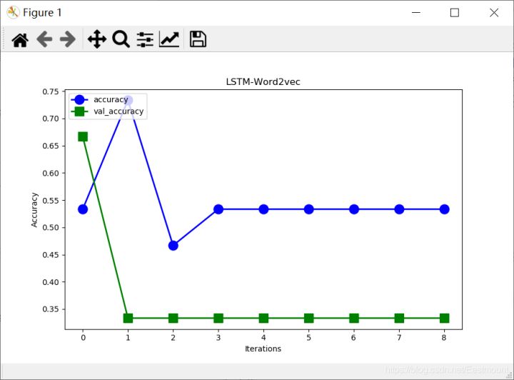
plt.title("LSTM-Word2vec")
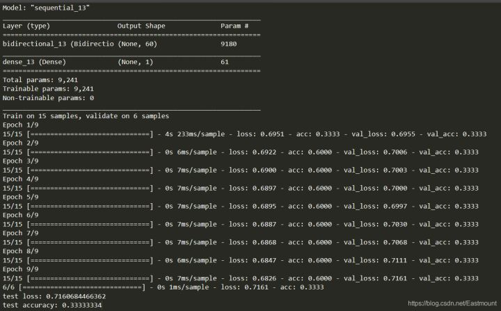
plt.show()The output results are shown below and are still not ideal.
- test loss: 0.712007462978363
- test accuracy: 0.33333334
Model: "sequential_22"
_________________________________________________________________
Layer (type)                 Output Shape              Param #
=================================================================
embedding_8 (Embedding)      (None, None, 128)         2560
_________________________________________________________________
lstm_8 (LSTM)                (None, 128)               131584
_________________________________________________________________
dense_21 (Dense)             (None, 1)                 129
=================================================================
Total params: 134,273
Trainable params: 134,273
Non-trainable params: 0
_________________________________________________________________
Train on 15 samples, validate on 6 samples
Epoch 1/9
15/15 [==============================] - 8s 552ms/sample - loss: 0.6971 - acc: 0.5333 - val_loss: 0.6911 - val_acc: 0.6667
Epoch 2/9
15/15 [==============================] - 5s 304ms/sample - loss: 0.6910 - acc: 0.7333 - val_loss: 0.7111 - val_acc: 0.3333
Epoch 3/9
15/15 [==============================] - 3s 208ms/sample - loss: 0.7014 - acc: 0.4667 - val_loss: 0.7392 - val_acc: 0.3333
Epoch 4/9
15/15 [==============================] - 4s 261ms/sample - loss: 0.6890 - acc: 0.5333 - val_loss: 0.7471 - val_acc: 0.3333
Epoch 5/9
15/15 [==============================] - 4s 248ms/sample - loss: 0.6912 - acc: 0.5333 - val_loss: 0.7221 - val_acc: 0.3333
Epoch 6/9
15/15 [==============================] - 3s 210ms/sample - loss: 0.6857 - acc: 0.5333 - val_loss: 0.7143 - val_acc: 0.3333
Epoch 7/9
15/15 [==============================] - 3s 187ms/sample - loss: 0.6906 - acc: 0.5333 - val_loss: 0.7346 - val_acc: 0.3333
Epoch 8/9
15/15 [==============================] - 3s 185ms/sample - loss: 0.7066 - acc: 0.5333 - val_loss: 0.7578 - val_acc: 0.3333
Epoch 9/9
15/15 [==============================] - 4s 235ms/sample - loss: 0.7197 - acc: 0.5333 - val_loss: 0.7120 - val_acc: 0.3333
6/6 [==============================] - 0s 43ms/sample - loss: 0.7120 - acc: 0.3333
test loss: 0.712007462978363
test accuracy: 0.33333334
The corresponding figure is shown below.
3.LSTM+TFIDF text classification
At the same time, supplement LSTM+TFIDF text classification code.
# -*- coding: utf-8 -*-
"""
Created on Sat Mar 28 22:10:20 2020
@author: Eastmount CSDN
"""
from jieba import lcut
from numpy import zeros
import matplotlib.pyplot as plt
from gensim.models import Word2Vec
from sklearn.model_selection import train_test_split
from tensorflow.python.keras.preprocessing.sequence import pad_sequences
from tensorflow.python.keras.models import Sequential
from tensorflow.python.keras.layers import Dense, LSTM, GRU, Embedding
from tensorflow.python.keras.callbacks import EarlyStopping
#-----------------------------------Define parameters----------------------------------
max_features = 20 #Word vector dimension
units = 30 #Number of RNN neurons
maxlen = 40 #Maximum length of sequence
epochs = 9 #Maximum rounds of training
batch_size = 12 #Data size of each batch
verbose = 1 #Training process display
patience = 1 #Training rounds without improvement
callbacks = [EarlyStopping('val_acc', patience=patience)]
#--------------------------------Loading data and preprocessing-------------------------------
data = [
[0, 'Millet porridge is a kind of porridge made of millet as the main ingredient. It has light taste and fragrance. It is simple and easy to make, good for the stomach and digestion'],
[0, 'When cooking porridge, be sure to boil water first, and then put in the washed millet'],
[0, 'Protein and amino acids, fat, vitamins, minerals'],
[0, 'Millet is a traditional healthy food, which can be stewed and porridge alone'],
[0, 'Apple is a kind of fruit'],
[0, 'Porridge has high nutritional value, rich in minerals and vitamins, rich in calcium, which helps to metabolize the excess salt in the body'],
[0, 'Eggs have high nutritional value and are high-quality protein B A good source of vitamins, but also provide fat, vitamins and minerals'],
[0, 'The apples in this supermarket are very fresh'],
[0, 'In the north, millet is one of the main foods, and many areas have the custom of eating millet porridge for dinner'],
[0, 'Millet has high nutritional value, comprehensive and balanced nutrition, and mainly contains carbohydrates'],
[0, 'Protein, amino acid, fat, vitamin and salt'],
[1, 'Xiaomi, Samsung and Huawei are the three flagship mobile phones of Android'],
[1, 'Forget about Xiaomi Huawei! Meizu mobile phone re exposure: This is really perfect'],
[1, 'Apple may return to 2016, but this time it can't raise prices significantly'],
[1, 'Samsung wants to continue to suppress Huawei, just by A70 not enough yet'],
[1, 'Samsung's mobile screen will reach a new high, surpassing Huawei and Apple's flagship'],
[1, 'Huawei P30,Samsung A70 Sold like hot cakes and won Suning's best mobile phone marketing award'],
[1, 'Lei Jun, tell you with a picture: where is the gap between Xiaomi and Samsung'],
[1, 'Xiaomi chat APP official Linux Version on-line, adaptive depth system'],
[1, 'Samsung has just updated its wearable device APP'],
[1, 'The cross-border between Huawei and Xiaomi is not terrible. It can't break the inner "ceiling"'],
]
#Chinese word segmentation
X, Y = [' '.join(lcut(i[1])) for i in data], [i[0] for i in data]
print(X)
print(Y)
#['when cooking porridge, be sure to boil water first, and then put in the washed millet',...]
#--------------------------------------Calculate word frequency------------------------------------
from sklearn.feature_extraction.text import CountVectorizer
from sklearn.feature_extraction.text import TfidfTransformer
#Convert words in text into word frequency matrix
vectorizer = CountVectorizer()
#Count the number of occurrences of a word
X_data = vectorizer.fit_transform(X)
print(X_data)
#Get all text keywords in the word bag
word = vectorizer.get_feature_names()
print('[View words]')
for w in word:
print(w, end = " ")
else:
print("\n")
#frequency matrix
print(X_data.toarray())
#Count the word frequency matrix X into TF-IDF value
transformer = TfidfTransformer()
tfidf = transformer.fit_transform(X_data)
#The view data structure tfidf[i][j] represents the TF IDF weight in class I text
weight = tfidf.toarray()
print(weight)
#Data set partition
X_train, X_test, y_train, y_test = train_test_split(weight, Y)
print(X_train.shape, X_test.shape)
print(len(y_train), len(y_test))
#(15, 117) (6, 117) 15 6
#--------------------------------Modeling and training-------------------------------
model = Sequential()
#Building the Embedding layer 128 represents the vector dimension of the Embedding layer
model.add(Embedding(max_features, 128))
#Build LSTM layer
model.add(LSTM(128, dropout=0.2, recurrent_dropout=0.2))
#Building a full connectivity layer
#Note that when building the LSTM layer above, you will only get the output of the last node. If you need to output the results at each time point, you need to return_sequences=True
model.add(Dense(units=1, activation='sigmoid'))
#Model visualization
model.summary()
#Activating neural network
model.compile(optimizer = 'rmsprop', #RMSprop optimizer
loss = 'binary_crossentropy', #Binary cross entropy loss
metrics = ['acc'] #Calculation error or accuracy
)
#train
history = model.fit(X_train, y_train, batch_size=batch_size, epochs=epochs,
verbose=verbose, validation_data=(X_test, y_test))
#----------------------------------Prediction and visualization------------------------------
#forecast
score = model.evaluate(X_test, y_test, batch_size=batch_size)
print('test loss:', score[0])
print('test accuracy:', score[1])
#visualization
acc = history.history['acc']
val_acc = history.history['val_acc']
# Set class label
plt.xlabel("Iterations")
plt.ylabel("Accuracy")
#mapping
plt.plot(range(epochs), acc, "bo-", linewidth=2, markersize=12, label="accuracy")
plt.plot(range(epochs), val_acc, "gs-", linewidth=2, markersize=12, label="val_accuracy")
plt.legend(loc="upper left")
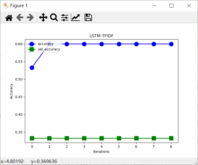
plt.title("LSTM-TFIDF")
plt.show()The output results are as follows:
- test loss: 0.7694947719573975
- test accuracy: 0.33333334
Model: "sequential_1"
_________________________________________________________________
Layer (type)                 Output Shape              Param #
=================================================================
embedding_1 (Embedding)      (None, None, 128)         2560
_________________________________________________________________
lstm_1 (LSTM)                (None, 128)               131584
_________________________________________________________________
dense_1 (Dense)              (None, 1)                 129
=================================================================
Total params: 134,273
Trainable params: 134,273
Non-trainable params: 0
_________________________________________________________________
Train on 15 samples, validate on 6 samples
Epoch 1/9
15/15 [==============================] - 2s 148ms/sample - loss: 0.6898 - acc: 0.5333 - val_loss: 0.7640 - val_acc: 0.3333
Epoch 2/9
15/15 [==============================] - 1s 48ms/sample - loss: 0.6779 - acc: 0.6000 - val_loss: 0.7773 - val_acc: 0.3333
Epoch 3/9
15/15 [==============================] - 1s 36ms/sample - loss: 0.6769 - acc: 0.6000 - val_loss: 0.7986 - val_acc: 0.3333
Epoch 4/9
15/15 [==============================] - 1s 47ms/sample - loss: 0.6722 - acc: 0.6000 - val_loss: 0.8097 - val_acc: 0.3333
Epoch 5/9
15/15 [==============================] - 1s 42ms/sample - loss: 0.7021 - acc: 0.6000 - val_loss: 0.7680 - val_acc: 0.3333
Epoch 6/9
15/15 [==============================] - 1s 36ms/sample - loss: 0.6890 - acc: 0.6000 - val_loss: 0.8147 - val_acc: 0.3333
Epoch 7/9
15/15 [==============================] - 1s 37ms/sample - loss: 0.6906 - acc: 0.6000 - val_loss: 0.8599 - val_acc: 0.3333
Epoch 8/9
15/15 [==============================] - 1s 43ms/sample - loss: 0.6819 - acc: 0.6000 - val_loss: 0.8303 - val_acc: 0.3333
Epoch 9/9
15/15 [==============================] - 1s 40ms/sample - loss: 0.6884 - acc: 0.6000 - val_loss: 0.7695 - val_acc: 0.3333
6/6 [==============================] - 0s 7ms/sample - loss: 0.7695 - acc: 0.3333
test loss: 0.7694947719573975
test accuracy: 0.33333334
The corresponding figure is as follows:
4. Comparative analysis of machine learning and deep learning
Finally, we make a simple comparison and find that machine learning is better than deep learning. Why? What improvements can we make?
- MultinomialNB+TFIDF: test accuracy = 0.67
- GaussianNB+Word2Vec: test accuracy = 0.83
- RNN+Word2Vector: test accuracy = 0.33333334
- LSTM+Word2Vec: test accuracy = 0.33333334
- LSTM+TFIDF: test accuracy = 0.33333334
The author makes a simple analysis based on the articles of the bosses and his own experience. The reasons are as follows:
- everything The reason for data set preprocessing is that the above codes do not filter stop words, and a large number of punctuation and stop words affect the effect of text classification. At the same time, the dimension setting of word vector also needs to be debugged.
- The second is Reason for dataset size. CNN is recommended when there is a small amount of data. The over fitting of RNN will make you cry without tears. If there is a large amount of data, perhaps the RNN effect will be better. For innovation, RLSTM and RCNN are good choices in recent years. However, if only for application, ordinary machine learning methods are good enough (especially news data sets). If considering the time cost, Bayesian is undoubtedly the real best choice.
- Three is CNN and RNN have different applicability. CNN is good at learning and capturing spatial features, and RNN is good at capturing temporal features. In terms of structure, RNN is better. Mainstream NLP problems, such as translation and text generation, and the introduction of seq2seq (two independent RNNs) broke through many previous benchmark s. The introduction of Attention is to solve the problem of long sentences. Its essence is to plug in an additional softmax to learn the mapping relationship between words. It is a bit like plug-in storage. Its root comes from a paper called "neural turning machine".
- Four is Different data sets adapt to different methods, and each method has its own advantages. Some emotional analysis GRU is better than CNN, while CNN may have advantages in news classification and text classification competition. CNN has the advantage of speed. On basically large data, CNN can increase parameters and fit more kinds of local phase frequencies to obtain better results. If you want to build a system and the two algorithms have their own advantages, it's time for ensemble s to come on stage.
- Five is In the field of text emotion classification, GRU is better than CNN, and this advantage of GRU will be further amplified with the growth of sentence length. When the emotional classification of a sentence is determined by the whole sentence, GRU will be easier to classify correctly. When the emotional classification of a sentence is determined by several local key phrases, CNN will be easier to classify correctly.
In short, in the real experiment, we try to choose the algorithm suitable for our data set, which is also a part of the experiment. We need to compare various algorithms, various parameters and various learning models to find a better algorithm. Subsequent authors will further study TextCNN, Attention, BiLSTM, GAN and other algorithms, and hope to make progress with you.
reference:
Thank you again for the contributions of the predecessors and teachers of the references. At the same time, I also refer to the author's Python artificial intelligence and data analysis series. Please download the source code in github.
[1] The imdb and MNIST datasets of Keras cannot be downloaded. Problem solved - golden youth v
[2] Official website example explanation 4.42 (imdb.py) - keras learning notes IV - wyx100
[3] Keras text classification - strongly push teacher Jiwei's articles
[4] TextCNN text classification (keras Implementation) - strong push for teacher Asia Lee's articles
[5] Keras text classification implementation - strong inference of Mr. Wang Yilei's article
[6 ]Introduction to natural language processing (II) – Keras implementation of BiLSTM+Attention news headline text classification - ilivecode
[7] Solving large-scale text classification problems with CNN RNN Attention - overview and practice - zhihuqingsong
[8] Text classification based on word2vec and CNN: Review & Practice - Niu Yafeng serena
[9] https://github.com/keras-team/keras
[10] [deep learning] keras's use and skills of EarlyStopping - zwqjoy
[11] Why is the validation accuracy greater than train accuracy in deep learning- ICOZ
[12] Keras implements CNN text classification - vivian_ll
[13] Keras text classification practice (Part I) - Weixin_ thirty-four million three hundred and fifty-one thousand three hundred and twenty-one
[14] Is CNN good or RNN good for Chinese long text classification- Know
Click focus to learn about Huawei cloud's new technologies for the first time~