Transferred from: (41 messages) explain PyTorch project in detail. Use tensorboardx for training visualization_ Shallow temple - CSDN blog_ tensorboardx

What is TensorboardX

Tensorboard is an additional tool of TensorFlow, which can record the digital, image and other contents of the training process, so as to facilitate researchers to observe the neural network training process. However, for other neural network training frameworks such as PyTorch, there are no similar tools with the same comprehensive functions as tensorboard. Some existing tools have limited functions or are difficult to use (tensorboard_logger, visdom, etc.). Tensorboard x is a tool that enables other neural network frameworks other than TensorFlow to use the convenient functions of tensorboard. The github warehouse of TensorboardX is here.

Configure TensorboardX

Environmental requirements

• Operating system: MacOS / Ubuntu (Windows not tested)
• Python2/3
• PyTorch >= 1.0.0 && torchvision >= 0.2.1 && tensorboard >= 1.12.0

The above version requires you to correspond TensorboardX@1.6 edition. In order to ensure the timeliness of the version, we recommend that you follow tensorboardx   README in github warehouse   Configure the environment according to the requirements of.

install

You can install directly using pip or from the source code.

Installing using pip

pip install tensorboardX

Install from source

git clone https://github.com/lanpa/tensorboardX && cd tensorboardX && python setup.py install

Using TensorboardX

First, you need to create an example of SummaryWriter:

#for instance
from tensorboardX import SummaryWriter

# Creates writer1 object.
# The log will be saved in 'runs/exp'
writer1 = SummaryWriter('runs/exp')

# Creates writer2 object with auto generated file name
# The log directory will be something like 'runs/Aug20-17-20-33'
writer2 = SummaryWriter()

# Creates writer3 object with auto generated file name, the comment will be appended to the filename.
# The log directory will be something like 'runs/Aug20-17-20-33-resnet'
writer3 = SummaryWriter(comment='resnet')

The above shows three methods to initialize SummaryWriter:

1. Provide a path that will be used to save the log (such as writer1 above)
2. No parameters, the default is   runs / date time   Path to save the log (such as writer2 above)
3. Provide a comment parameter that will use   runs / datetime - Comment   Path to save the log (such as writer3 above)

Generally speaking, we create a SummaryWriter with different paths for each experiment, which is also called a run, such as runs/exp1 and runs/exp2.

Next, we can call various add_something methods of the SummaryWriter instance to write different types of data to the log. To view and visualize these data in the browser, just open tensorboard on the command line:

tensorboard --logdir=<your_log_dir>

Note: in the above command, < your_log_dir > can be the path of a single run, such as runs/exp generated by writer1 above, or the parent directory of multiple runs, such as runs / below, there may be many subfolders, and each folder represents an experiment.

              By making -- logdir=runs /, we can easily compare the data obtained from different experiments under runs / horizontally in the tensorboard visual interface.

Use various add methods to record data

The following describes various data recording methods of the SummaryWriter instance in detail, and provides corresponding examples for reference. (you can run tests)

Digital (scalar)

use   add_scalar   Method to record numeric constants.

add_scalar(tag, scalar_value, global_step=None, walltime=None)

parameter

tag (string): Data name. Data with different names are displayed by different curves
scalar_value (float): Numeric constant value
global_step (int, optional): Trained step
walltime (float, optional): Record the time of occurrence,Default to time.time()

It should be noted that the scalar_value here must be of float type. If it is a PyTorch scalar tensor, you need to call the. item() method to obtain its value. We generally use the add_scalar method to record the changes of loss, accuracy, learning rate and other values in the training process, so as to intuitively monitor the training process.

Example:

from tensorboardX import SummaryWriter
writer = SummaryWriter('runs/scalar_example')
for i in range(10):
    writer.add_scalar('quadratic', i**2, global_step=i)
    writer.add_scalar('exponential', 2**i, global_step=i)

Here, we are in a path for   runs/scalar_example   The quadratic function data is written in the run of   quadratic   And exponential function data   Exponential, the effect of the original blogger in the browser visual interface is as follows:

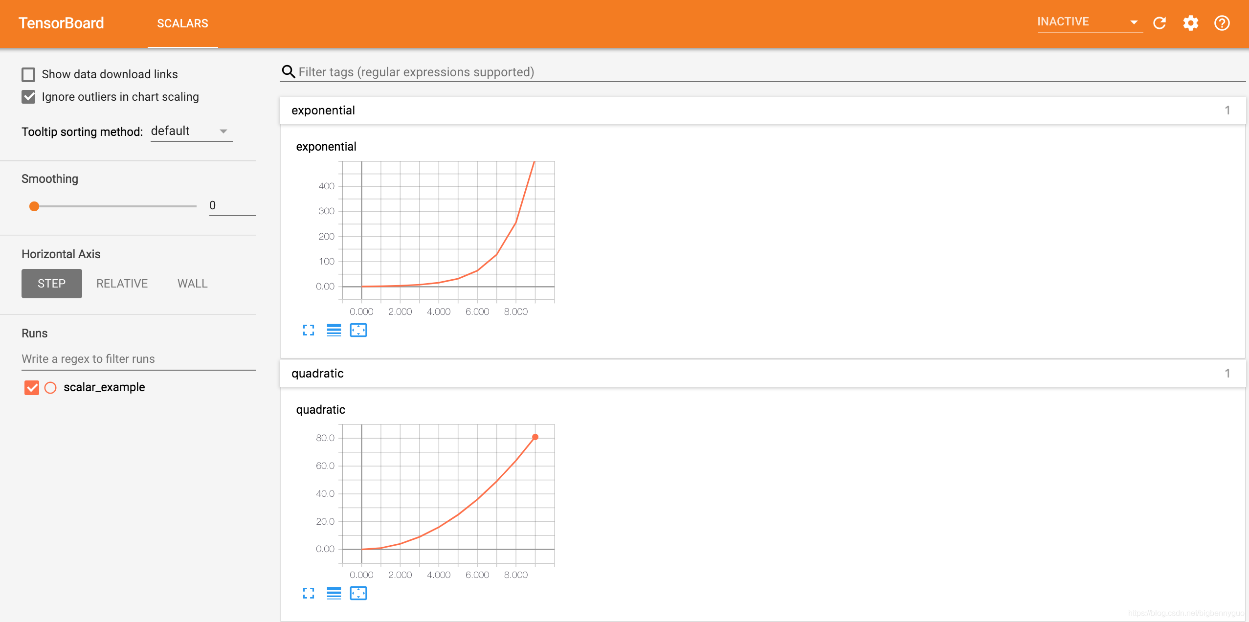
  But in my local area, there is no curve (my corresponding version is: tensorboard = = 2.6.0, tensorflow = = 2.6.2, Torch = = 1.10.0, torch vision = = 0.11.1, OS is win10, please let me know)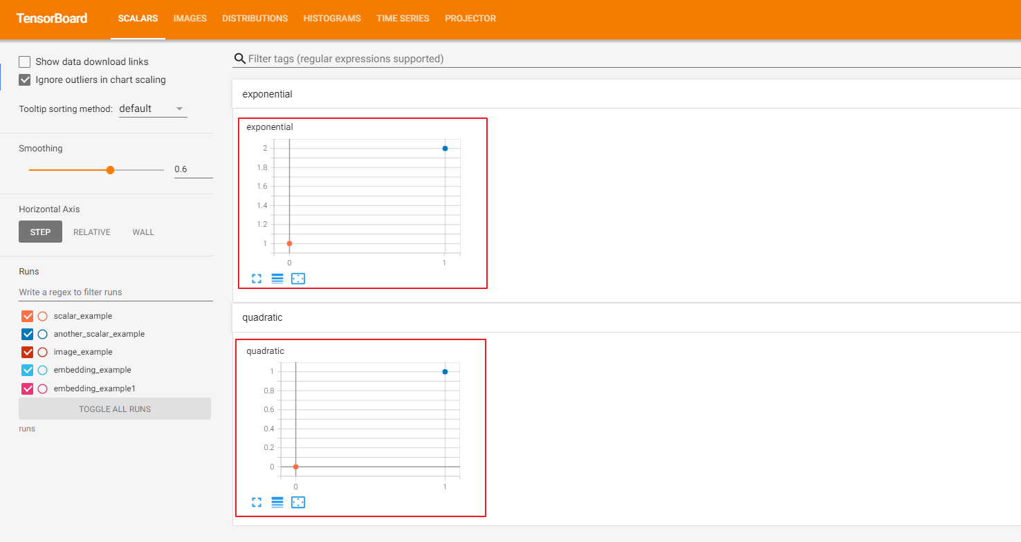

  Create a new python file as follows

from tensorboardX import SummaryWriter

writer = SummaryWriter('runs/another_scalar_example')
for i in range(10):
    writer.add_scalar('quadratic', i**3, global_step=i)
    writer.add_scalar('exponential', 3**i, global_step=i)

Next, we write quadratic function and exponential function data with the same name but different parameters in another run with the path of runs / other_scalar_example. The visualization effect is as follows. We find that the quantities with the same name are displayed in the same chart for comparison observation. At the same time, we can also select which runs to view in the runs column on the left side of the screen Data.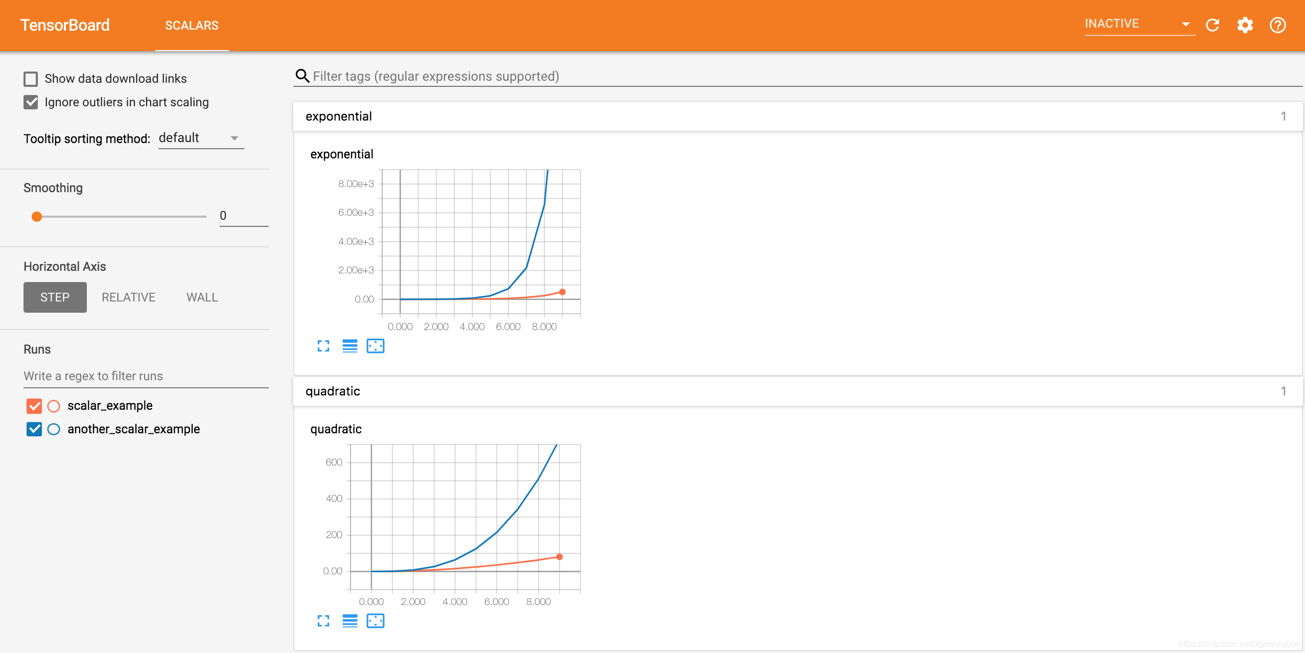

Picture (image)

use   add_image   Method to record single image data. Note that this method requires   pillow   Library support.

add_image(tag, img_tensor, global_step=None, walltime=None, dataformats='CHW')

Parameters:

tag (string): Data name
img_tensor (torch.Tensor / numpy.array): image data
global_step (int, optional): Trained step
walltime (float, optional): Record the occurrence time. The default value is time.time()
dataformats (string, optional): The format of image data. The default is 'CHW'，Namely Channel x Height x Width，It can also be 'CHW','HWC' or 'HW' etc.

We usually use   add_image   To observe the generation effect of generative model in real time, or visualize the results of segmentation and target detection to help debug the model.

Example

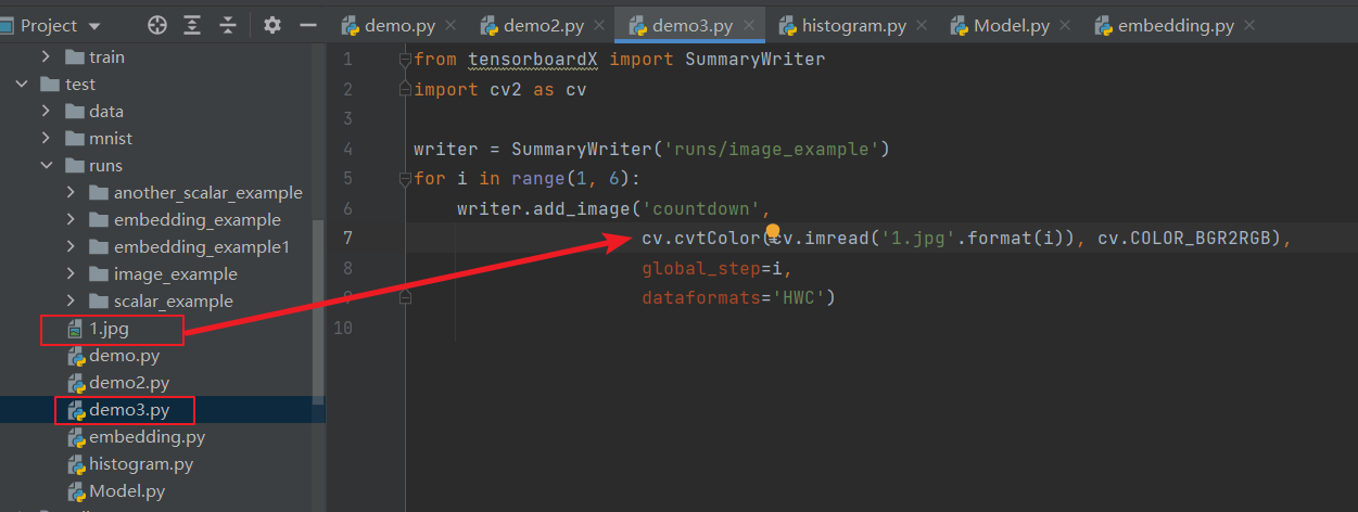
from tensorboardX import SummaryWriter
import cv2 as cv

writer = SummaryWriter('runs/image_example')
for i in range(1, 6):
    writer.add_image('countdown',
                     cv.cvtColor(cv.imread('{Your own image file name [I put it in the same path as the current file, you can choose the absolute path] is shown below}.jpg'.format(i)), cv.COLOR_BGR2RGB),
                     global_step=i,
                     dataformats='HWC')

For example, the current python asking price is demo3, the picture is 1.jpg, and the directory structure is as follows:

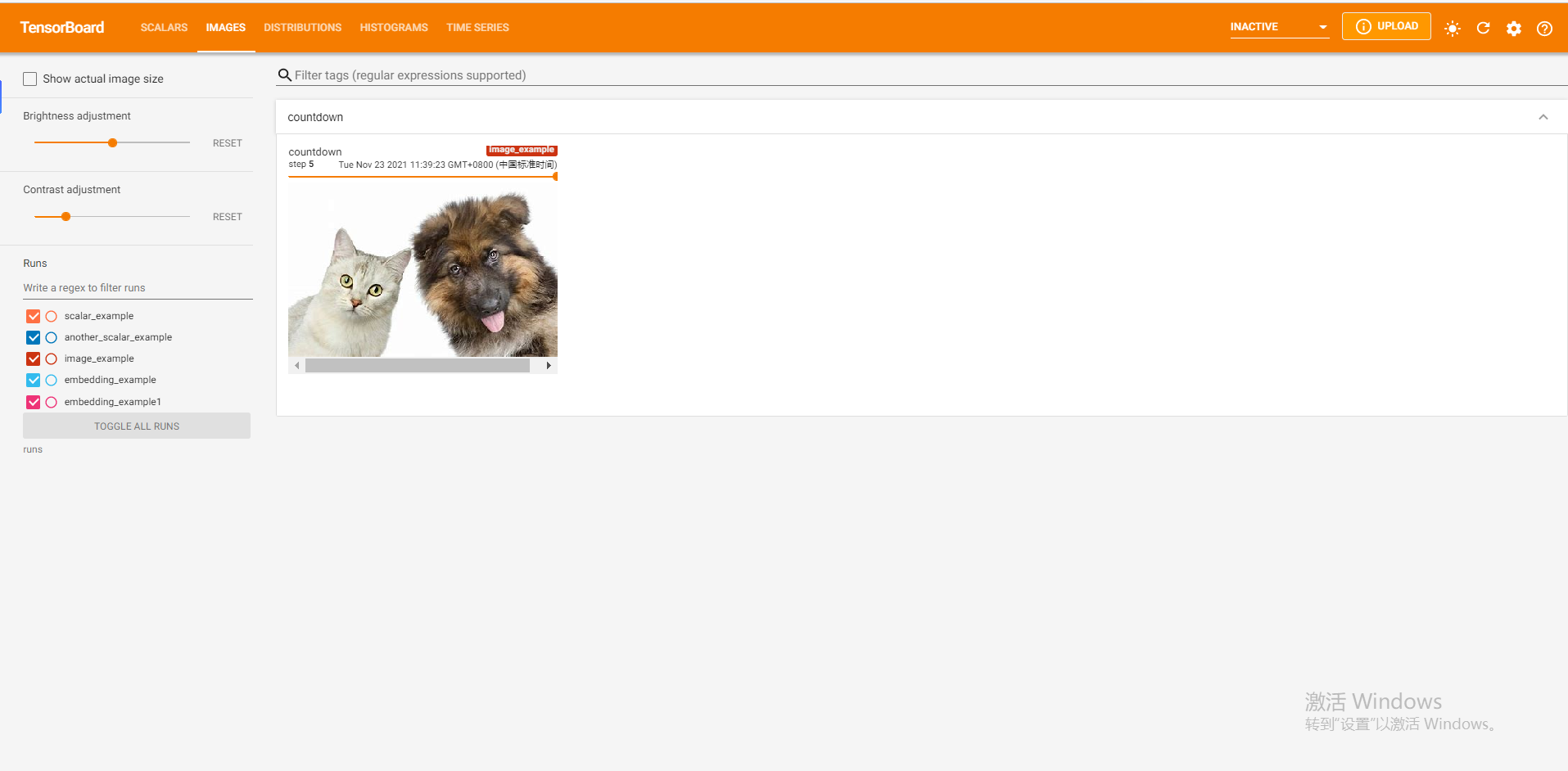
The add_image method can only insert one picture at a time. If you want to insert more than one picture at a time, there are two methods:

1. use   torchvision   Medium   make_grid   method   [official documents]   Assemble multiple pictures into one picture, and then call   add_image   method.
2. use   SummaryWriter   of   add_images   method   [official documents] , parameters and   add_image   Similarly, it will not be introduced separately here.

Histogram

use   add_histogram   Method to record a histogram of a set of data.

add_histogram(tag, values, global_step=None, bins='tensorflow', walltime=None, max_bins=None)

parameter

tag (string): Data name
values (torch.Tensor, numpy.array, or string/blobname): Data used to construct histograms
global_step (int, optional): Trained step
bins (string, optional): Values are 'tensorflow','auto','fd' etc., This parameter determines the way to divide buckets，See details here. 
walltime (float, optional): Record the occurrence time. The default value is time.time()
max_bins (int, optional): Maximum barrels

We can understand their approximate distribution by observing the histogram of data, training parameters and features, so as to assist the training process of neural network.

Example

from tensorboardX import SummaryWriter
import numpy as np

writer = SummaryWriter('runs/embedding_example')
writer.add_histogram('normal_centered', np.random.normal(0, 1, 1000), global_step=1)
writer.add_histogram('normal_centered', np.random.normal(0, 2, 1000), global_step=50)
writer.add_histogram('normal_centered', np.random.normal(0, 3, 1000), global_step=100)

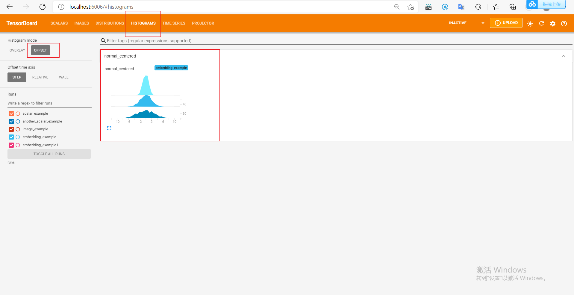
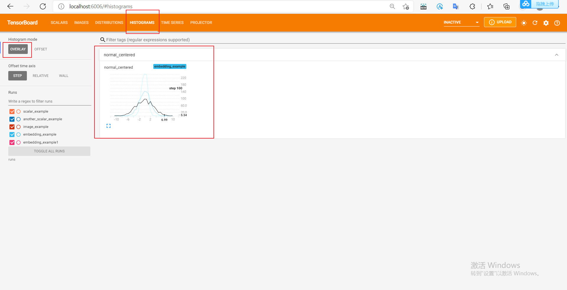
We use numpy to sample from the normal distribution of different variances. After opening the browser visualization interface, we will find that there are two more columns "DISTRIBUTIONS" and "HISTOGRAMS", which are used to observe the data distribution. In "HISTOGRAMS", the HISTOGRAMS of the same data with different step s can be offset or overlapped As shown in the following figure, the first figure is the "DISTRIBUTIONS" interface, and the second and third are the "HISTOGRAMS" interface.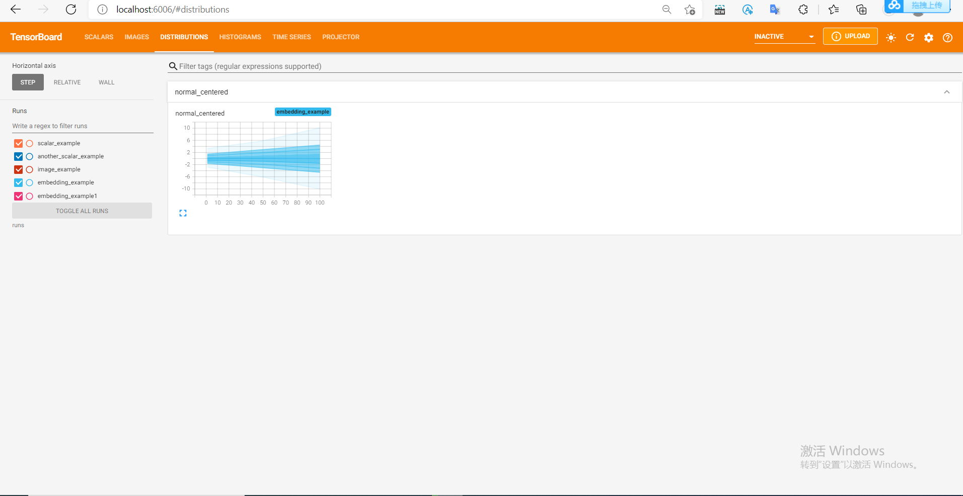

  The histograms of the same data at different step s can be offset or overlay: they correspond to the following two figures respectively

Operation diagram (graph)

use   add_graph   Method to visualize a neural network.

add_graph(model, input_to_model=None, verbose=False, **kwargs)

parameter

model (torch.nn.Module): Network model to be visualized
input_to_model (torch.Tensor or list of torch.Tensor, optional): The variable or group of variables to be input into the neural network

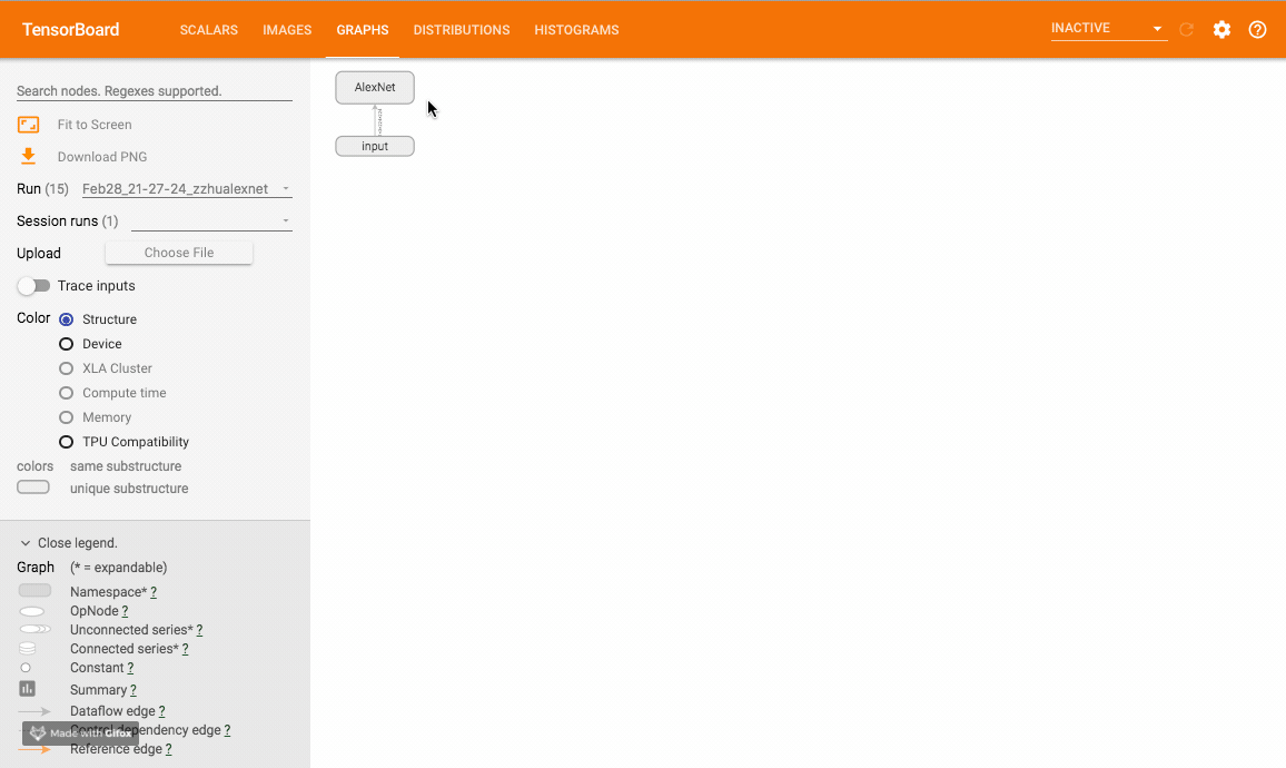
This method can visualize the neural network model, and TensorboardX gives an example Official sample You can try. The sample operation effect is as follows:

Embedding vector

use   add_embedding   Method can visualize embedding vectors in two-dimensional or three-dimensional space.

parameter

mat (torch.Tensor or numpy.array): A matrix, each row represents a data point in the feature space
metadata (list or torch.Tensor or numpy.array, optional): A one-dimensional list, mat Of each row of data in the label，Size should be and mat Same number of rows
label_img (torch.Tensor, optional): A shape such as NxCxHxW Tensor, corresponding mat The image displayed by each line of data, N Should and mat Same number of rows
global_step (int, optional): Trained step
tag (string, optional): Data name. Data with different names will be displayed separately

add_embedding is a very practical method. It can not only reduce the dimension of high-dimensional features to two-dimensional plane or three-dimensional space by using PCA, t-SNE and other methods, but also observe the K-nearest neighbor of each data point in the feature space before dimensionality reduction. In the following example, we take 100 data from MNIST training set, expand the image into one-dimensional vector, directly use it as embedding, and use TensorboardX to visualize it. (the following is the original blogger's code, but there is an error during runtime, which may be a version problem)

from tensorboardX import SummaryWriter
import torchvision

writer = SummaryWriter('runs/embedding_example')
mnist = torchvision.datasets.MNIST('mnist', download=True)
writer.add_embedding(
    mnist.train_data.reshape((-1, 28 * 28))[:100,:],
    metadata=mnist.train_labels[:100],
    label_img = mnist.train_data[:100,:,:].reshape((-1, 1, 28, 28)).float() / 255,
    global_step=0
)

Modified code:

from tensorboardX import SummaryWriter
import torchvision

writer = SummaryWriter('runs/embedding_example1')
mnist = torchvision.datasets.MNIST('mnist', download=True)
writer.add_embedding(
    mnist.data.reshape((-1, 28 * 28))[:100,:],
    metadata=mnist.targets[:100],
    label_img = mnist.data[:100,:,:].reshape((-1, 1, 28, 28)).float() / 255,
    global_step=0
)

The visualization effect in three-dimensional space after PCA dimensionality reduction is as follows:

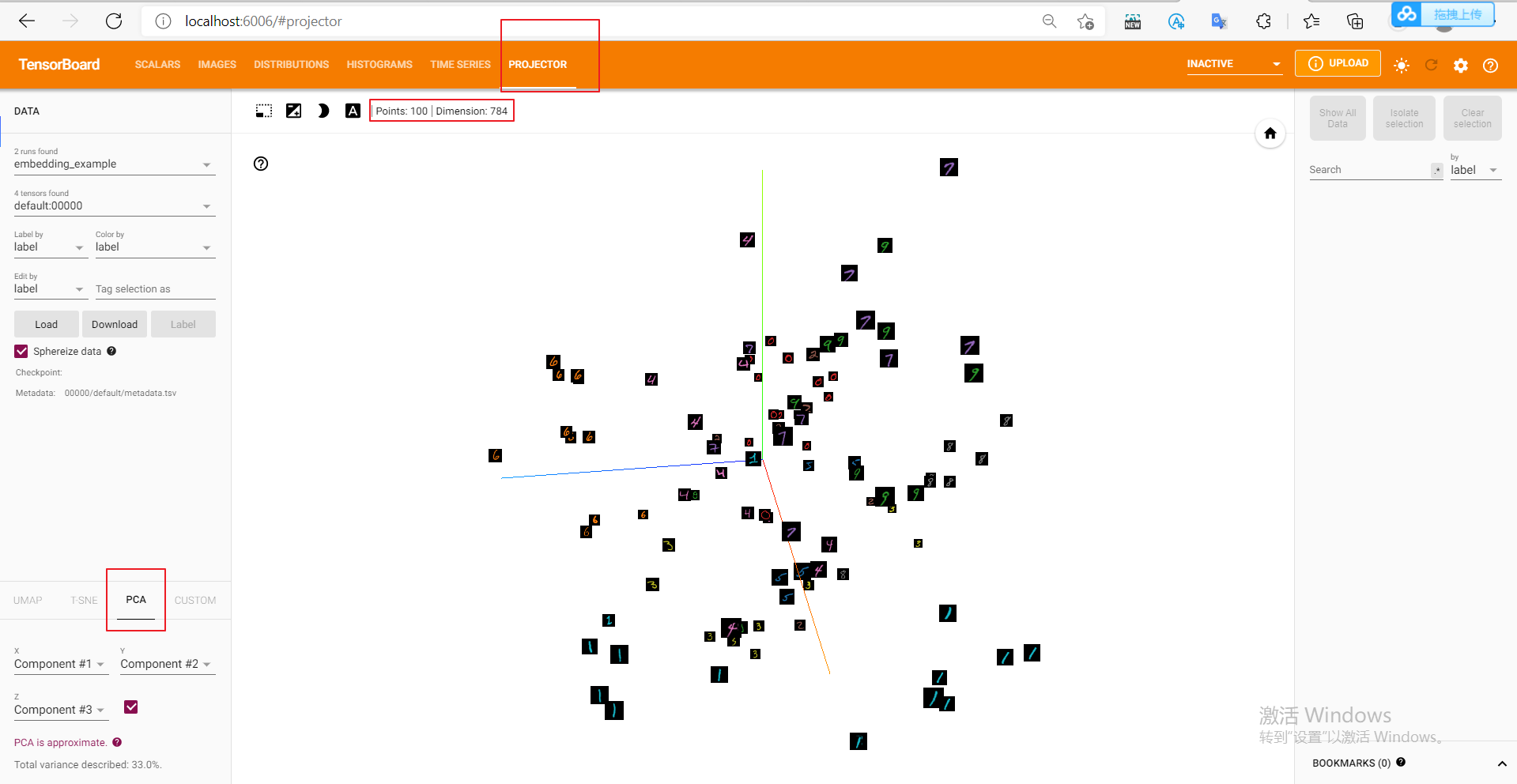
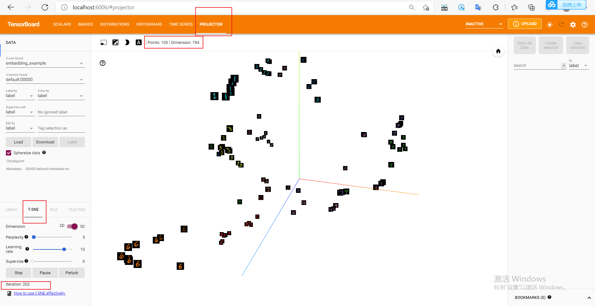
  It can be found that although no feature extraction has been done, MNIST data has shown the effect of clustering, and the distance between the same numbers is closer (did you think of KNN classifier). We can also click on the bottom left   t-SNE, visualization with t-SNE method.

  add_embedding   Points needing attention in the method:

mat It's two-dimensional MxN，metadata It's one-dimensional N，label_img It's four-dimensional NxCxHxW!
label_img Remember to normalize to 0-1 Between float value

other

TensorboardX has many other methods besides the common methods mentioned above, such as   add_audio,add_figure   And so on, interested friends can refer to [official documents] . I believe that after reading this article, you can skillfully call other methods by analogy.

Some tips
(1) If you get stuck when entering the embedding visual interface, please update the tensorboard to the latest version (> = 1.12.0).
(2) The tensorboard has a cache. If you delete some run folders, you'd better restart the tensorboard to avoid invalid data interfering with the display effect.
(3) If you do not see the effect in the web page visualization interface in real time after performing the add operation, try restarting tensorboard.
--------