This paper mainly uses keras to make a regression prediction on some Boston house price data sets, The code architecture is the same as before (only multi-layer perceptron is used): network models for data preprocessing, network framework building, compilation, cyclic training and test training. Except that data preprocessing is slightly different from the previous regression model, others are basically similar. However, in the regression prediction code of this paper, cross validation, a commonly used training method when there are few data sets, will be mentioned.

Regression prediction of house prices, that is, select the factors affecting house prices, quantify them, then use the data and the corresponding house prices to train the neural network, and finally use the quantitative value of factors to predict the trend of house prices.

In the Boston house price data set in Keras, there are only 506 samples, of which only 404 are used for training. Others are used for testing. Each sample has 13 characteristics, that is, there are 13 factors affecting house prices (some of the 13 factors are specific values and some are given weight values). Therefore, the training data set is: [404,13].

       1. Data preprocessing

First, use keras to import the required packages and data sets

from keras.datasets import boston_housing
(train_data,train_targets),(test_data,test_targets)=boston_housing.load_data()

Then the data are standardized to obtain the data with characteristic mean value of 0 and standard deviation of 1, which is more conducive to the processing and convergence of the network.

mean = train_data.mean(axis=0)  
train_data -= mean  
std = train_data.std(axis=0) 
train_data/=std 

test_data-=mean
test_data/=std

　

Train in the first part of the code_ data. Mean (axis=0) means train_ The std of the characteristic average value of each row in data is also the standard deviation of each row, that is, the 13 influencing factors in each group of data are labeled. (use print(train_data.shape) to get the shape of training data [404,13], axis=0 in the above code refers to 404)

In the second part of the code, we directly use the characteristic mean and standard deviation obtained from the training set to standardize the test set. The reason is that the network can not know the data of the test set in advance.

       2. Build network architecture

model=models.Sequential()
model.add(layers.Dense(32,activation='relu',input_shape=(trian_data.shape[1],)))
model.add(layers.Dense(32,activation='relu'))
model.add(layers.Dense(1))

The construction of the network architecture is the same as that in the previous article, but in the end, there is no need to carry out nonlinear processing, because changing the network requires a prediction, so you can directly output the value obtained by the network.

       3. compile

model.compile(
        optimizer='rmsprop',loss='mse',metrics=['mae'] )

The loss function used here is mae, that is, the average absolute error, that is, the square of the error between the predicted value and the real value is taken as the error obtained by the network for return training.

       4. Cyclic network

k=4
num=len(trian_data)//k
num_epochs=60
all_list=[]
for i in range(k):
    print('proccesing #',i)
    val_data=trian_data[i*num:(i+1)*num]
    val_target=trian_target[i*num:(i+1)*num]

    par_data=np.concatenate(
        [trian_data[:i*num],
        trian_data[(i+1)*num:]],
        axis=0
    )
    par_target=np.concatenate(
        [trian_target[:i*num],
        trian_target[(i+1)*num:]],
        axis=0
    )
           his=model.fit(par_data,par_target,epochs=num_epochs,batch_size=1,validation_data=(val_data,val_target))
    history=his.history['mae']
    all_list.append(history)

Because the data set is very rare (404), in order to improve the network performance, cross verification is used to strengthen the network performance. Cross verification is to divide all training data into n points, select one of them as the verification set and the rest as the test set in order until all N data have been verified. As shown in the figure below:

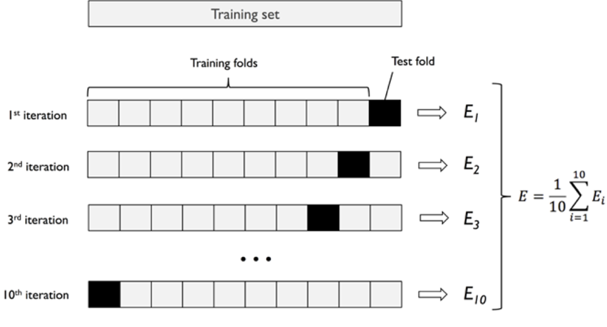
In the code, k is used to represent the total number of shares, and then it is verified. A total of k verifications are required, and num will be run each time_ Epochs times. Finally, save the mae value of each time in all_list for later drawing.

In the above code, because one has trained K (k=4) rounds, 60 times per round (epochs=60), we calculate the mean value of 60 times (four groups of data in total, calculate the mean value, and get 60 values from 4 * 60 values), and then use the obtained mean value to draw the graph. The code is as follows:

ave_list=[np.mean([x[i] for x in all_list]) for i in range(num_epochs)]
plt.plot(range(1,len(ave_list)+1),ave_list)
plt.xlabel('epochs')
plt.ylabel('validation mae')
plt.show()

The first line of code is to calculate the mean value of 60 epochs for the data in 4 groups respectively; The remaining code is the verification value curve of mae, and the obtained curve is shown in the figure:

 

 

 

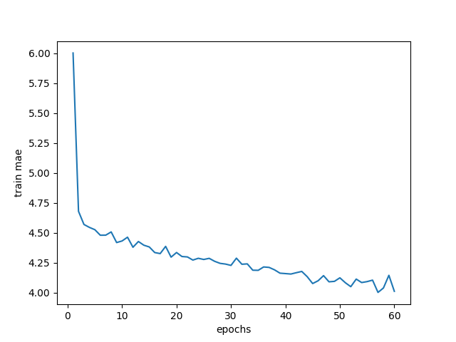
The smaller the mae, the more accurate the prediction is; Other curves, such as the loss value curve of the verification set, only need to replace {4 history in circular network:

#Before replacement
history=his.history['mae']
#After replacement
history=his.history['val_mae']

After that, you can change the name of the y-axis, about what curve you can draw, because in model In fit, we use the training set and verification set, so we finally get the loss and mae of the training set and the loss and mae of the verification set.

　　5. All codes

from keras.datasets import boston_housing
from keras import layers
from keras import models
import numpy as np
import matplotlib.pyplot as plt
(train_data,train_target),(tesr_data,test_target)=boston_housing.load_data()
print(train_data[1])
mean=np.mean(train_data)
train_data-=mean
str=np.std(train_data)
train_data/=str

tesr_data-=mean
tesr_data/=str
print(train_data[1])

model=models.Sequential()
model.add(layers.Dense(32,activation='relu',input_shape=(train_data.shape[1],)))
model.add(layers.Dense(32,activation='relu'))
model.add(layers.Dense(1))
model.compile(
        optimizer='rmsprop',loss='mse',metrics=['mae'] )


k=4
num=len(train_data)//k
num_epochs=60
all_list=[]
for i in range(k):
    print('proccesing #',i)
    val_data=train_data[i*num:(i+1)*num]    #Extract the validated data from the training set
    val_target=train_target[i*num:(i+1)*num]    #Extract the verified label part (house price) from the training set

    par_data=np.concatenate(        #Glue the rest of the training data together
        [train_data[:i*num],
        train_data[(i+1)*num:]],
        axis=0
    )
    par_target=np.concatenate(      #Glue the rest of the training label together
        [train_target[:i*num],
        train_target[(i+1)*num:]],
        axis=0
    )
    his=model.fit(par_data,par_target,epochs=num_epochs,batch_size=1,validation_data=(val_data,val_target))
    history=his.history['mae']
    all_list.append(history)


ave_list=[np.mean([x[i] for x in all_list]) for i in range(num_epochs)]
plt.plot(range(1,len(ave_list)+1),ave_list)
plt.xlabel('epochs')
plt.ylabel('train mae')
plt.show()

At present, all the network layers used are multi-layer perceptron, that is, neural network algorithm. The convolution neural network algorithm will be introduced in the later article.