In order to complete the design, I recently started the introductory deep learning

I would like to share with you my notes when reading the fish book. If there is any omission, please correct it!

If reprinted, please indicate the source!

1, Perceptron

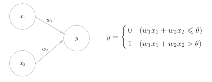
The perceptron receives multiple input signals and outputs one signal.

As shown in the figure, the sensor receives two input signals. Where \ (\ theta \) is the threshold, and neurons will be activated if they exceed the threshold.

The limitation of perceptron is that it can only represent the space divided by a straight line, that is, linear space. Multi layer perceptron can realize complex functions.

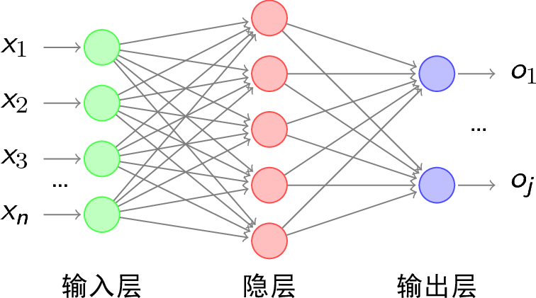
2, Neural network

Neural network consists of three parts: input layer, hidden layer and output layer

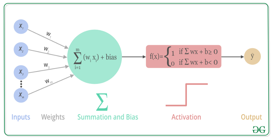
1. Activate function

The activation function converts the sum of input signals into output signals, which is equivalent to simple screening and processing of calculation results.

The activation function shown in the figure is a step function.

1) sigmoid function

sigmoid function is a commonly used neural network activation function.

The formula is:

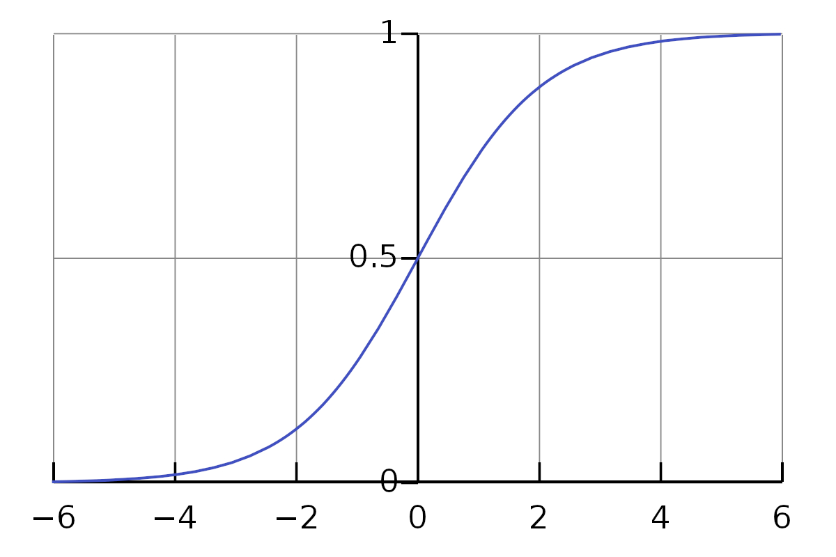
As shown in the figure, its output value is between 0 and 1.

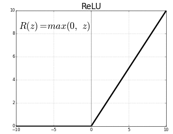
2) ReLU function

The ReLU(Rectified Linear Unit) function is a recently used activation function.

3) tanh function

2. Implementation of three-layer neural network

The neural network includes: input layer, two hidden layers and output layer.

def forward(network, x): # x is the input data
  # For the processing of the first hidden layer, point multiplication plus offset is transmitted to the activation function
  a1 = np.dot(x, W1) + b1
  z1 = sigmoid(a1)
  # Processing of the second hidden layer
  a2 = np.dot(z1, W2) + b2
  z2 = sigmoid(a2)
  #Output layer processing identity_ Function as is output a3
  a3 = np.dot(z2, W3) + b3
  y = identify_function(a3)
  return y # y is the final result

3. Output layer activation function

Generally speaking, the regression problem chooses the identity function, and the classification problem chooses the softmax function.

Formula of softmax function:

Assuming that there are \ (n \) neurons in the output layer, calculate the output \ (y_{k} \) of the \ (K \) th neuron.

The sum of the output values of the softmax function is 1. Therefore, we can interpret its output as probability.

The number of neurons in the output layer is generally equal to the number of set categories.

4. Handwritten numeral recognition

Use MNIST dataset.

Using pickle package to serialize and deserialize the required data can speed up the reading speed.

Normalization: limit the data to a certain range.

Batch batch

The input data is packaged in batches, and multiple pictures can be processed at one time.

batch_size = 100
for in range(0, len(x), batch_size) # x is the input data
	x_batch = x[i:i+batch_size] # Slice processing, batch at a time_ Size picture
  y_batch = predict(network, x_batch)
  p = np.argmax(y_batch, axis = 1)

3, Learning of neural network

Learning refers to the process of automatically obtaining the optimal weight parameters from the training process.

1. Data driven mode

Extract feature quantities (SIFT, SURF or HOG) from the image, use these feature quantities to convert the image data into vectors, and then use SVM, KNN and other classifiers in machine learning to learn the converted vectors.

2. Loss function

The neural network takes the loss function as an index to find the optimal weight parameters.

The purpose of neural network learning is to reduce the value of loss function as much as possible.

We generally use mean square error and cross entropy error functions.

1) Mean square error

Mean Squared Error.

\(Y {k} \) represents the output result of neural network, \ (t {k} \) represents the correct unlabeling, and \ (k \) represents the data dimension.

One hot means: the correct solution label is expressed as 1, and other labels are expressed as 0.

For example:

t = [0, 0, 1, 0, 0, 0, 0, 0, 0, 0] # It is assumed that the number "2" is the correct result during number recognition
y = [0.1, 0.05, 0.6, 0.0, 0.05, 0.1, 0.0, 0.1, 0.0, 0.0]

2) Cross entropy error

Cross Entropy Error

\(Y {K} \) represents the output result of the neural network, and \ (t {K} \) represents the correct unlabeling.

3) Mini batch learning

If we require the average loss function of all training data, taking the cross entropy error as an example, it is:

We can choose a part from all the data as the representative of all the data. This part is mini batch.

Like a sample survey.

train_size = x_train.shape[0] # Number of all data in the training set
batch_size = 10 #Size of mini batch
batch_mask = np.random.choice(train_size, batch_size)#The function starts from train_size number randomly selected batch_size number
x_batch = x_train[batch_mask] 
t_batch = t_train[batch_mask]

3. Numerical differentiation

1) Derivative

The central difference is used to approximate the derivative.

def numerical_diff(f, x) #Find the derivative of function f(x) at X
	h = 1e-4 #Tiny value
  return (f(x+h)-f(x-h)) / (2 * h)

2) Gradient

The vector formed by the partial derivatives of all variables is called gradient.

For example, for the function \ (f(x,y)=x^2+y^2 \), the gradient at \ ((x,y) \) is \ (\ frac{\partial f}{\partial x},\frac{\partial f}{\partial y}) \)

Its Python implementation is as follows:

def numerical_gradient(f, x):
  h = 1e-4
  grad = np.zeros_like(x) #Generate an empty array with the same size as the variable group x to store the gradient
 	
  for idx in range(x.size):
    tmp_val = x[idx]
    # f(x+h)
    x[idx] = tmp_val + h
    fxh1 = f(x)
    # f(x-h)
    x[idx] = tmp_val - h
    fxh2 = f(x)
    # Calculate the partial derivative of x[idx]
    grad[idx] = (fxh1 - fxh2) / (2*h)
    x[idx] = tmp_val # Restore value

The gradient points to the direction where the function value at each point decreases the most.

3) Gradient descent method

We usually use the gradient descent method to find the minimum value of the loss function along the gradient direction.

Take the function mentioned above as an example, use the following formula to continuously update the gradient value:

\(\ eta \) is an update quantity called learning rate. The initial value of learning rate is generally 0.01 or 0.001

The gradient descent method is implemented in Python as follows:

# f is the function, init_x is the initial variable group, the learning rate is 0.01, and the cycle is 100 times
def gradient_descent(f, init_x, learning_rate = 0.01, step_num = 100):
  x = init_x
  for i in range(step_num):
    grad = numerical_gradient(f, x)
    x = x - lr*grad
  return x

4. Gradient of neural network

The learning of neural network requires the gradient of loss function with respect to weight parameters.

For example, for a 2 * 3 weight parameter \ (W \), the loss function is \ (L \), then the gradient \ (\ frac{\partial L}{\partial W} \) is:

5. Implementation of learning algorithm

The process of dynamically adjusting weights and offsets to fit training data is called learning. There are four steps:

• Mini batch: select Mini batch data with the goal of reducing the value of its loss function. Random gradient descent method SGD.
• Calculate gradient: calculate the gradient of each weight parameter
• Update parameter: slightly update the weight along the gradient direction
• Repeat the above steps

Suppose a neural network has two weight parameters \ (W1 \) and \ (W2 \), two bias parameters \ (b1 \), $b2 $:

class TwoLayerNet:
  # Calculates and returns the network output value
  def predict(self, x):
    a1 = np.dot(x, W1) + b1
    z1 = sigmoid(a1)
    a2 = np.dot(z1, W2) + b2
    y = softmax(a2)
    return y
  # Calculate the loss value t as the correct solution label
  def loss(self, x, t):
    y = self.predict(x)
    return cross_entropy_error(y, t)
  # Calculated gradient
  def count_gradient(self, x, t):
    loss_W = lambda W: self.loss(x, t)
    # Calculate gradient and other parameters ellipsis
    grads['W1'] = numerical_gradient(loss_W, params['W1'])

Implementation of mini batch:

# Super parameter
iters_num = 10000 # Number of drops
train_size = x_train.shape[0]
batch_size = 100
learning_rate = 0.1
network = TwoLayerNetwork(input_size = 784, hidden_size = 50, output_size = 10)
for i in range(iters_num):
  # Get Mini batch
  batch_mask = np.random.choice(train_size, batch_size)
  x_batch = x_train[batch_mask]
  t_batch = t_train[batch_mask]
  # Calculated gradient
  grad = network.count_gradient(x_batch, t_batch)
  # Update parameters
  for key in ('W1','b1','W2','b2'):
    network.params[key] -= leraning_rate * grad[key]

An epoch represents the number of updates when all training data have been used in learning.

4, Error back propagation method BP

The gradient of weight parameters can be calculated quickly by error back propagation method.

It is based on the chain rule.

• The back propagation of the addition node outputs the upstream value to the downstream intact.
• The back propagation of the multiplication node is multiplied by the flip value of the input signal.

1. Implementation of activation function layer

1) ReLU

class Relu:
  def __init__(self):
    self.mask = None
  # Forward propagation
  def forward(self, x):
    self.mask = (x <= 0)
    out = x.copy()
    out[self.mask] = 0
    return out
  # Back propagation
  def backward(self,dout):
    dout[self.mask] = 0
    dx = dout
    return dx

2) sigmoid

class Sigmoid:
  def __init__(self):
    self.out = None
  # Forward propagation
  def forward(self, x):
    out = 1 / (1 + np.exp(-x))
    self.out = out
    return out
  # Back propagation
  def backward(self, dout):
    dx = dout * (1.0 - self.out) * self.out
    return dx

2. Implementation of affine / softmax layer

1) Affine

The forward propagation process of neural network is to calculate the weighted sum according to the input data, weight and bias, and output it to the next layer after passing through the activation function.

The matrix product operation is called Affine transformation in the field of geometry, so we implement the processing of Affine transformation as Affine layer.

class Affine:
  def __init__(self, W, b):
    self.W = W
    self.b = b
    self.x = None
    self.dW = None
    self.db = None
  # Forward propagation
  def forward(self, x):
    self.x = x
    out = np.dot(x, self.W) + self.b
    return out
  # Back propagation
  def backward(self, dout):
    dx = np.dot(dout, self.W.T)
    self.dW = np.dot(self.x.T, dout)
    self.db = np.sum(dout, axis = 0)
    return dx

2) Softmax

The softmax function normalizes the input value and outputs it. Considering that the cross entropy error as a loss function is also included here, it is called softmax with loss layer.

class SoftmaxWithLoss:
  def __init__(self):
    self.loss = None
    self.y = None
    self.t = None
  # Forward propagation 
  def forward(self, x, t):
    self.t = t
    self.y = softmax(x)
    self.loss = cross_entropy_error(self.y, self.t)
    return self.loss
  # Back propagation
  def backward(self, dout = 1):
    batch_size = self.t.shape[0]
    dx = (self.y - self.t) / batch_size
    return dx

5, Learning related skills

1. Parameter update

The learning purpose of neural network is to find the parameters that make the value of loss function as small as possible. This process is called Optimization

Common methods include SGD, Momentum, AdaGrad and Adam.

1) SGD

Random gradient descent method.

class SGD:
  def __init__(self, lr = 0.01):
    self.lr = lr
  
  def update(self, params, grads):
    for key in params.keys():
      params[key] -= self.lr * grads[key]

2) Momentum

The disadvantage of SGD method is that the direction of gradient does not have the direction of minimum ambition. Momentum means momentum.

The mathematical formula is as follows:

Indicates that the object is under force in the gradient direction.

class Momentum:
  def __init__(self, lr = 0.01, momentum = 0.9):
    self.lr = lr
    self.momentum = momentum
    self.v = None
  
  def update(self, params, grads):
    if self.v is None:
      self.v = {}
      for key, val in params.items():
        self.v[key] = np.zeros_like(val)
    for key in params.keys():
      self.v[key] = self.momentum * self.v[key] - self.lr * grads[key]
      params[key] += self.v[key]

3) AdaGrad

The AdaGrad method retains the sum of squares of all previous gradient values and will adjust the learning rate appropriately for each element of the parameter.

Ada stands for Adaptive

class AdaGrad:
  def __init__(self, lr = 0.01):
    self.lr = lr
    self.h = None
  
  def update(self, params, grads):
    if self.h is None:
      self.h = {}
      for key, val in params.items():
        self.h[key] = np.zeros_like(val)
    for key in params.keys():
      self.h[key] += grads[key] * grads[key]
      params[key] -= self.lr * grads[key] / (np.sqrt(self.h[key]) + 1e-7)

4) Adam

Adam is a recent parameter update method, which will set three super three places.

2. Initial value of weight

The distribution of activation values of each layer requires an appropriate breadth, otherwise the gradient may disappear.

1) Xavier initial value

In the general deep learning framework, Xavier initial value has been used as a standard.

In the Xavier initial value, if the number of nodes in the previous layer is \ (n \), the initial value uses the distribution with the standard deviation of \ (\ frac{1}{\sqrt{n} \).

node_num = 100
w = np.random.randn(node_num, node_num) / np.sqrt(node_num)

2) He initial value of relu

When the activation function uses ReLU, the initial value of He is generally used.

If the number of nodes in the previous layer is \ (n \), the initial value uses a Gaussian distribution with a standard deviation of \ (\ sqrt{\frac{2}{n} \).

3. Batch Normalization

In order to make the distribution of activation values of each layer have appropriate breadth, the Batch Normalization method is used for forced adjustment.

Therefore, we need to insert a Batch Norm layer between the affinity layer and the activation function layer. Regularization is carried out in the unit of mini batch during learning.

Calculate the mean value \ (\ mu B \) and variance \ (\ Sigma {B} ^ 2 \) of the set of \ (n \) input data of mini batch \ (b = {x {1}, X {2},..., X {m}} \).

4. Inhibition of over fitting

Over fitting is a very common problem in machine learning. Over fitting refers to the state that only the training data can be fitted, but other data not included in the training data can not be well fitted.

Therefore, we need some methods to suppress overfitting. Weight attenuation is one of the methods.

1) Weight attenuation

For all weights, the weight attenuation method will add \ (\ frac{1}{2}\lambda W^2 \) to the loss function, that is, the \ (L2 \) norm of the weight.

Therefore, in the calculation of the weight gradient, the derivative \ (\ lambda W \) of the regularization term should be added to the result of the previous error back propagation method.

2) Dropout

When the network model is complex, the Dropout method is used to suppress over fitting.

Dropout is a method of deleting neurons during learning. During training, the neurons in the hidden layer are randomly selected and deleted. The deleted neurons no longer transmit signals.

class Dropout:
  def __init__(self, dropout_ratio = 0.5):
    self.dropout_ratio = dropout_ratio
    self.mask = None
  
  def forward(self, x, train_flg = True):
    if train_flg:
      self.mask = np.random.rand(*x.shape) > self.dropout_ratio
      return x * self.mask
    else:
      return x * (1.0 - self.dropout_ratio)
  
  def backward(self, dout):
    return dout * self.mask

5. Verification of super parameters

The super parameters include the number of neurons, batch size, learning rate and so on.

We cannot use test data to evaluate the performance of superparameters, otherwise it will cause over fitting

When adjusting the super parameter, the special confirmation data for the super parameter must be used, which is called validation data

6, Convolutional neural network

The structure of CNN can be assembled like building blocks. Among them, there are Convolution layer and Pooling layer.

In CNN, the connection order of layers is: Revolution - relu - pooling

Pooling is sometimes omitted.

1. Convolution layer

In the full connection layer, the shape of data is ignored. The convolution layer can keep the shape unchanged. When the input data is an image, the convolution layer receives the input data in the form of three-dimensional data and outputs it to the next time in the form of three-dimensional data.

The input and output data of convolution layer is called Feature Map.

1) Convolution operation

Convolution is equivalent to a filter.

The filter is the weight W in the output.

The filter will extract the original information such as edges or patches.

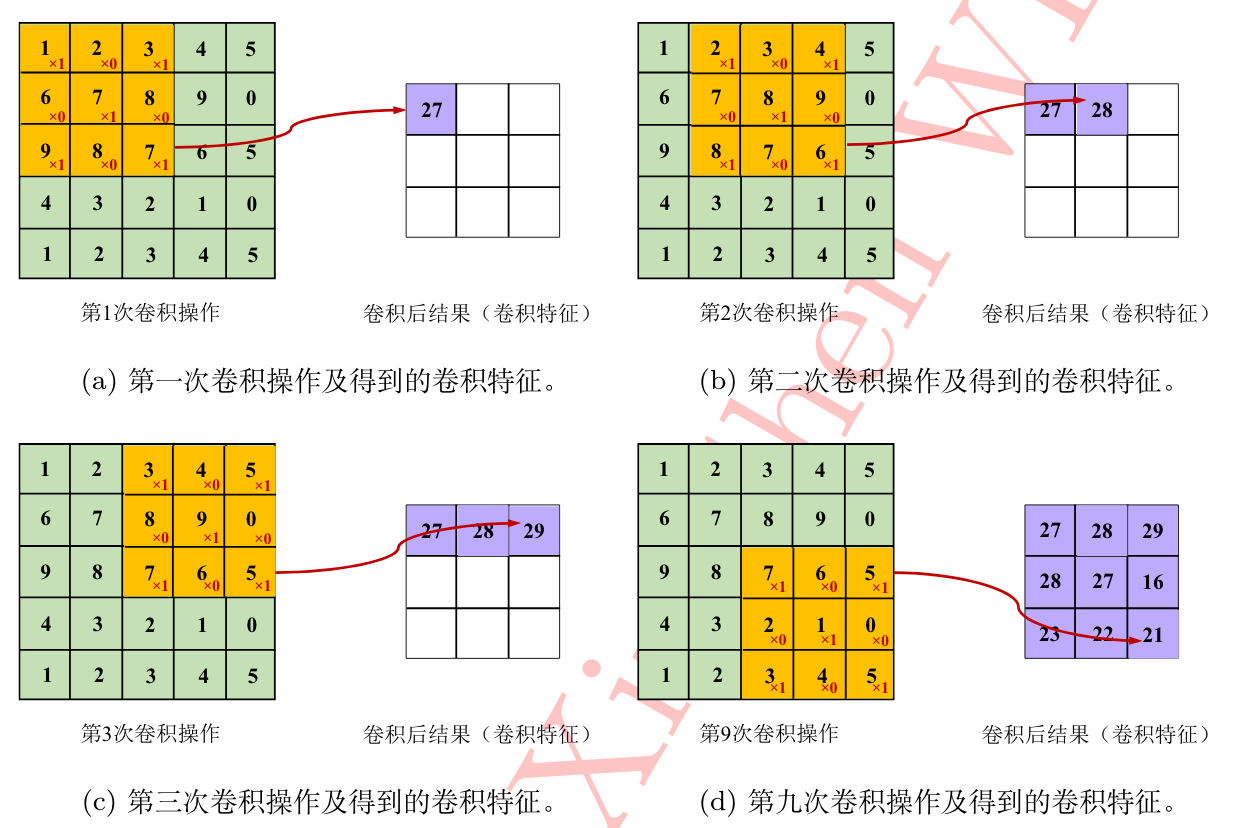
As shown in the figure, the input data size is \ ((5,5) \), the filter size is \ ((3,3) \), and the output size is \ ((3,3) \).

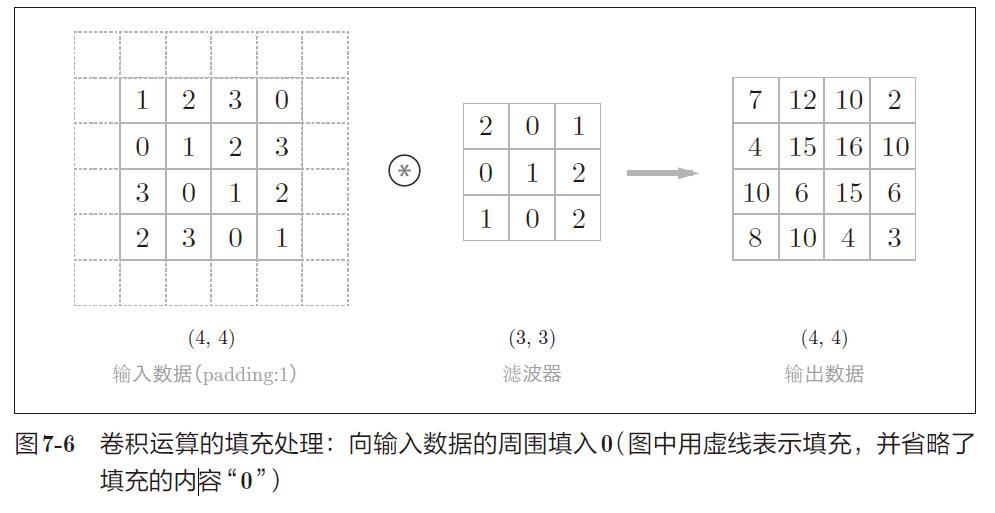
2) Padding

Before convolution layer processing, it is sometimes necessary to fill fixed data around the input data to expand the data.

Filling is mainly used to adjust the size of the output.

3) Stride

The position interval to which the filter is applied is called the stride.

After increasing the stride, the output table is small; After increasing the filling, the stride changes.

Suppose the input size is \ ((H,W) \), the filter size is \ ((FH,FW) \), the output size is \ ((OH,OW) \), the filling is \ (P \), and the step is \ (S \).

Then the output size is:

4) Convolution operation of three-dimensional data

Taking the 3-channel RGB image as an example, the feature map in the depth direction is increased. When there are multiple characteristic images in the channel direction, the convolution operation of input data and filter will be carried out according to the channel, and the results will be added.

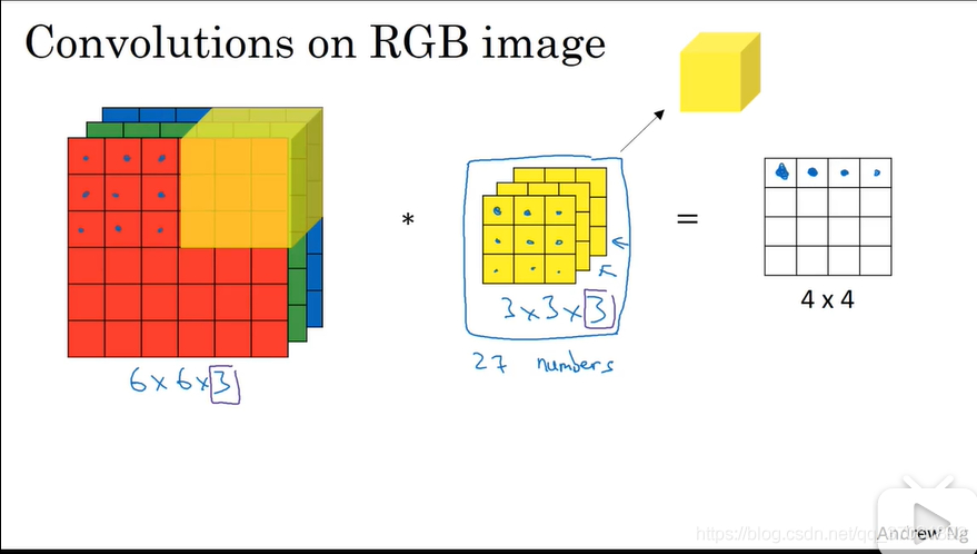
The number of channels of input data and the number of channels of filter should be the same.

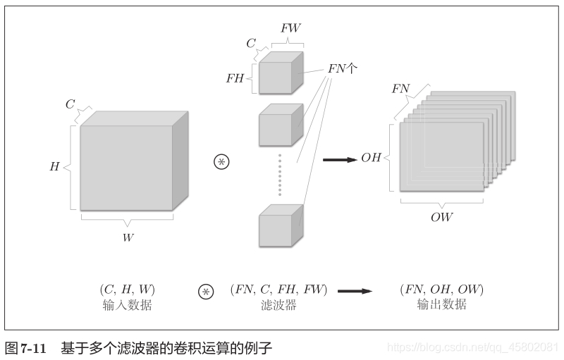
When there are multiple filters, the output characteristic diagram also has multiple layers.

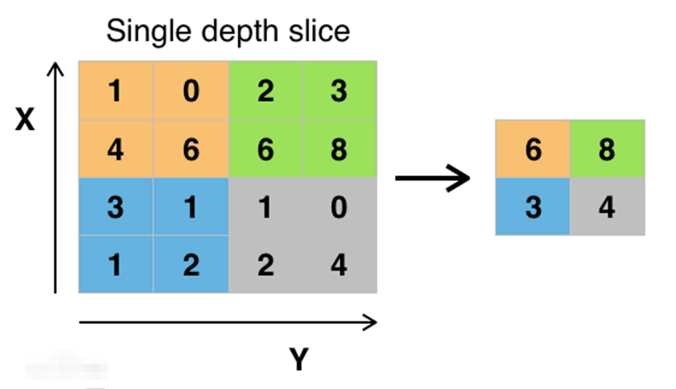
2. Pool layer

Pooling is a spatial operation that reduces the height and rectangle upward. In short, pooling is used to streamline data.

The operation that gets the maximum value on the Max pool. Generally speaking, the size of the pooled window will be the same as the stride.

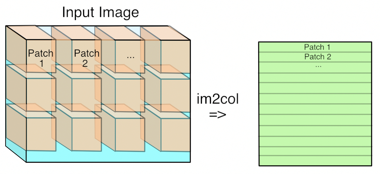
3. Implementation of convolution layer and pooling layer

A key function is im2col. It expands the input three-dimensional data into a two-dimensional matrix to fit the filter.

1) Convolution layer

class Convolution:
  def __init__(self, W, b, stride = 1, pad = 0):
    self.W = W
    self.b = b
    self.stride = stride
    self.pad = pad
  
  def forward(self, x)
  FN, C, FH, FW = self.W.shape # Number of filters, number of channels, height and length
  N, C, H, W = x.shape # Number of input data, number of channels, height and length
  # Calculate the length and height of the output data
  out_h = int(1 + (H + 2 * self.pad - FH) / self.stride) 
  out_w = int(1 + (W + 2 * self.pad - FW) / self.stride)
  # Convert 3D data to matrix using im2col
  col = im2col(x, FH, FW, self.stride, self.pad)
  col_W = self.W.reshape(FN, -1).T
  out = np.dot(col, col_W) + self.b # Multiply by weight and add cheap
  
  out = out.reshape(N, out_h, out_w, -1).transpose(0, 3, 1, 2) # Change back to 3D data
  return out

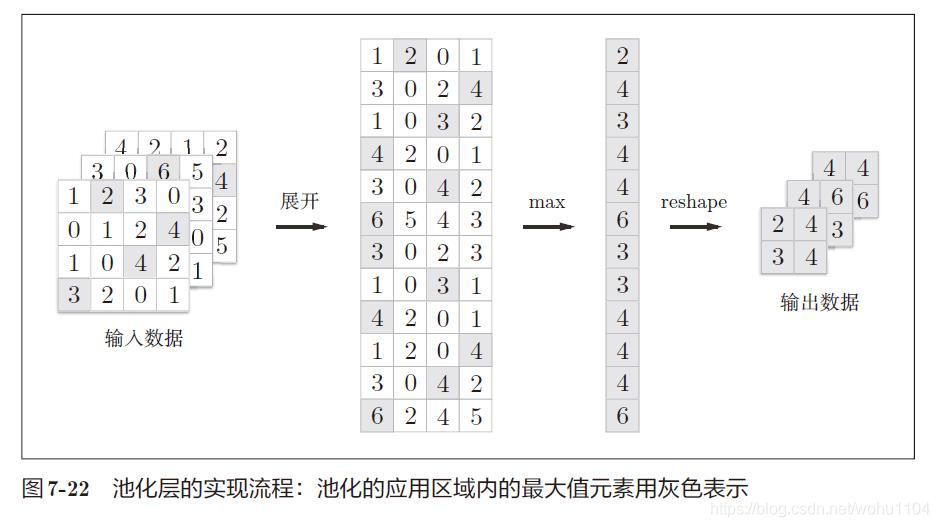
2) Pool layer

class Pooling:
  def __init__(self, pool_h, pool_w, stride = 1, pad = 0):
    self.pool_h, self.pool_w, self.stride, self.pad = pool_h, pool_w, stride, pad
  
  def forward(self, x):
    N, C, H, W = x.shape
    # Calculate the length and height of the output data
  	out_h = int(1 + (H - self.pool_h) / self.stride) 
  	out_w = int(1 + (W - self.pool_w) / self.stride)
    # open
    col = im2col(x, self.pool_h, self.pool_w, self.stride, self.pad)
    col = col.reshape(-1, self.pool_h * self.pool_w)
    # Maximum
    out = np.max(col, axis = 1)
    # transformation
    out = out.reshape(N, out_h, out_w, C).transpose(0, 3, 1, 2)
    return out

4. Implementation of MNIST digital recognition neural network

CN for handwritten numeral recognition

class SimpleConvNet:
    def __init__(self, input_dim = (1, 28, 28), conv_param = {'filter_num':30, 'filter_size':5, 'pad':0, 'stride':1}, hidden_size = 100, output_size = 10, weight_init_std = 0.01):
        """
        :param input_dim: Number and length of input data channels
        :param conv_param: Parameters of convolution layer, number of filters, dimension, filling and stride
        :param hidden_size: Number of hidden layer neurons
        :param output_size: Number of neurons in output layer
        :param weight_init_std: Initialization weight standard deviation
        """
        filter_num = conv_param['filter_num']
        filter_size = conv_param['filter_size']
        filter_pad = conv_param['pad']
        filter_stride = conv_param['stride']
        input_size = input_dim[1]
        conv_output_size = (input_size - filter_size + 2 * filter_pad) / filter_stride + 1
        pool_output_size = int(filter_num * (conv_output_size / 2) * (conv_output_size / 2))

        self.params = {'W1': weight_init_std * np.random.randn(filter_num, input_dim[0], filter_size, filter_size),
                       'b1': np.zeros(filter_num),
                       'W2': weight_init_std * np.random.randn(pool_output_size, hidden_size),
                       'b2': np.zeros(hidden_size),
                       'W3': weight_init_std * np.random.randn(hidden_size, output_size),
                       'b3': np.zeros(output_size)}
        self.layers = OrderedDict()
        self.layers['Conv1'] = Convolution(self.params['W1'], self.params['b1'], self.params['stride'], self.params['pad'])
        self.layers['ReLU1'] = Relu()
        self.layers['Pool1'] = Pooling(pool_h=2, pool_w=2, stride=2)
        self.layers['Affine1'] = Affine(self.params['W2'], self.params['b2'])
        self.layers['ReLU2'] = Relu()
        self.layers['Affine2'] = Affine(self.params['W3'], self.params['b3'])
        self.last_layer = SoftmaxWithLoss()

    def predict(self, x):
        for layer in self.layers.values():
            x = layer.forward(x)
        return x

    def loss(self, x, t):
        y = self.predict(t)
        return self.last_layer.forward(y, t)

    # Back propagation gradient
    def gradient(self, x, t):
        # forward
        self.loss(x, t)
        # backward
        dout = 1
        dout = self.last_layer.backward(dout)

        layers = list(self.layers.values())
        layers.reverse()
        for layer in layers:
            dout = layer.backward(dout)
        grads = {'W1': self.layers['Conv1'].dW, 'b1': self.layers['Conv1'].db, 'W2': self.layers['Affine1'].dW,
                 'b2': self.layers['Affine1'].db, 'W3': self.layers['Affine2'].dW, 'b3': self.layers['Affine2'].db}
        return grads