theta of Greek options( Θ)

preface

The previous article introduced the delta of option Greek value, and analyzed it to introduce the delta of option Greek value.

1, theta( Θ)

Theta is the partial derivative of option price to time, which can be understood as the rate of change of option price with time. When other conditions remain unchanged, the partial derivative of option price to time (T-t) is calculated as

For call options, Θ The calculation formula of call is:

For put options, Θ The calculation formula of input is:

Of which:

It can be seen from the formula that the value of put option Θ Than the corresponding call option Θ Higher than rKe^(-r (T-t)).

Theta( Θ) Used to describe the change rate of portfolio value over time, Θ Sometimes called combined time loss, i.e. time decay.

II Θ Relationship with the underlying asset price

one Θ Relationship between call and St

First, we define the functions required in this chapter (similar to the previous chapter)

# theta
import numpy as np
import scipy.stats as st
from matplotlib import cm
import math
import numpy as np
import matplotlib as mpl
import matplotlib.pyplot as plt
import mpl_toolkits.mplot3d.axes3d as p3
from scipy.integrate import quad

# Define the probability density function of standard normal distribution
def dN(x):
    '''Probability density function formula of standard normal distribution'''
    return math.exp(-0.5*x**2)/math.sqrt(2*math.pi)
def N(d):
    '''Calculate probability density function'''
    return quad(lambda x:dN(x),-20,d,limit=50)[0]
def d1f(St, K, t, T, r, sigma):
    '''BS In the model d1'''
    d1=(math.log(St/K)+(r+0.5*sigma**2)*(T-t))/(sigma*math.sqrt(T-t))
    return d1

# theta defining options
def call_theta(St, K, t, T, r, sigma):
    '''European call options theta'''
    d1 = d1f(St, K, t, T, r, sigma)
    d2 = d1 - sigma * math.sqrt(T - t)
    call_theta = -(St * dN(d1) * sigma / (2 * math.sqrt(T - t)) +
              r * K * math.exp(-r * (T - t)) * N(d2))
    return call_theta
def put_theta(St, K, t, T, r, sigma):
    '''European put options theta'''
    d1 = d1f(St, K, t, T, r, sigma)
    d2 = d1 - sigma * math.sqrt(T - t)
    put_theta = -St * dN(d1) * sigma / (2 * math.sqrt(T - t))+r * K * math.exp(-r * (T - t)) * N(-d2)
    return put_theta

The above code defines theta of European call option and put option
Next, the relationship between European call option theta and the underlying asset price is discussed

t=0
T=1
r=0.015
sigma=0.2
K1=2.6
K2=2.7
K3=2.8
K4=2.9
price=np.arange(1.4,4,0.01)

theta=[call_theta(St, K1, t, T, r, sigma) for St in price]
theta_1=[call_theta(St, K2, t, T, r, sigma) for St in price]
theta_2=[call_theta(St, K3, t, T, r, sigma) for St in price]
theta_3=[call_theta(St, K4, t, T, r, sigma) for St in price]
plt.figure(figsize=(12, 8))

# Call option
plt.plot(price, theta,  label="K=2.6")
plt.plot(price, theta_1, label="K=2.7")
plt.plot(price, theta_2, label="K=2.8")
plt.plot(price, theta_3, label="k=2.9")
plt.xlabel('stock value')
plt.ylabel("call_theta value")
plt.title('call_theta value of different strike option')
plt.grid()
plt.legend()

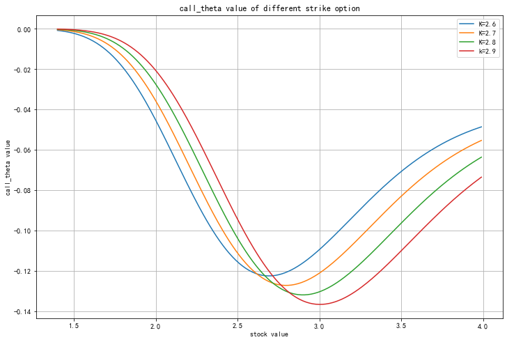
The results are shown in the figure. As can be seen from the figure, for call, Θ Always less than 0. That is, as the maturity date approaches, options become less and less valuable.

In addition, when the underlying asset price of the call option is very low, the price of the option is very low Θ Close to 0, corresponding to a parity call option, its Θ Very large and negative. When the price of the underlying asset is very high, Θ close to

Moreover, with the increase of exercise price, the price of parity option increases Θ Smaller and smaller.

two Θ Relationship between put and St

# Put option
t=0
T=1
r=0.015
sigma=0.2
K1=2.6
K2=2.7
K3=2.8
K4=2.9
price = np.arange(0.2, 5.8, 0.001)
put_theta_0=[put_theta(St, K1, t, T, r, sigma) for St in price]
put_theta_1=[put_theta(St, K2, t, T, r, sigma) for St in price]
put_theta_2=[put_theta(St, K3, t, T, r, sigma) for St in price]
put_theta_3=[put_theta(St, K4, t, T, r, sigma) for St in price]

plt.figure(figsize=(12, 8))
plt.plot(price, put_theta_0,label="K=2.6")
plt.plot(price, put_theta_1,label="K=2.7")
plt.plot(price, put_theta_2,label="K=2.8")
plt.plot(price, put_theta_3,label="K=2.9")

plt.xlabel('stock value')
plt.ylabel("put_theta value")
plt.title('put_theta value of different strike option')
plt.grid()
plt.legend()

plt.axhline(0,color='r',linestyle="--",alpha=0.8)  # Add y-axis reference line

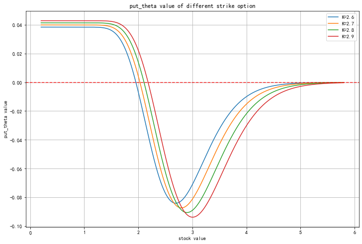
It can be seen from the figure below that for put options, when the option is within the depth price, i.e. s < < K, the value of the option Θ It could be positive.

Compared with real value option and imaginary value option, the negative value of parity option Theta is the largest.

III Θ Relationship with due days

one Θ Relationship between call and T

# Call option
St=2.7
T = np.arange(0.01, 1, 0.001)
call_theta_0=[call_theta(St, K1, t, T, r, sigma) for T in T]
call_theta_1=[call_theta(St, K2, t, T, r, sigma) for T in T]
call_theta_2=[call_theta(St, K3, t, T, r, sigma) for T in T]

# Drawing
plt.figure(figsize=(12, 8))
plt.grid()
plt.xlabel('T')
plt.ylabel("call_theta value")
plt.title('call_theta value of different T')
plt.grid()
plt.legend(loc=1)
# Call option
plt.plot(T, call_theta_0,  label="ITM/K=2.6")
plt.plot(T, call_theta_1, label="ATM/K=2.7")
plt.plot(T, call_theta_2, label="OTM/K=2.8")
plt.grid()
plt.legend()

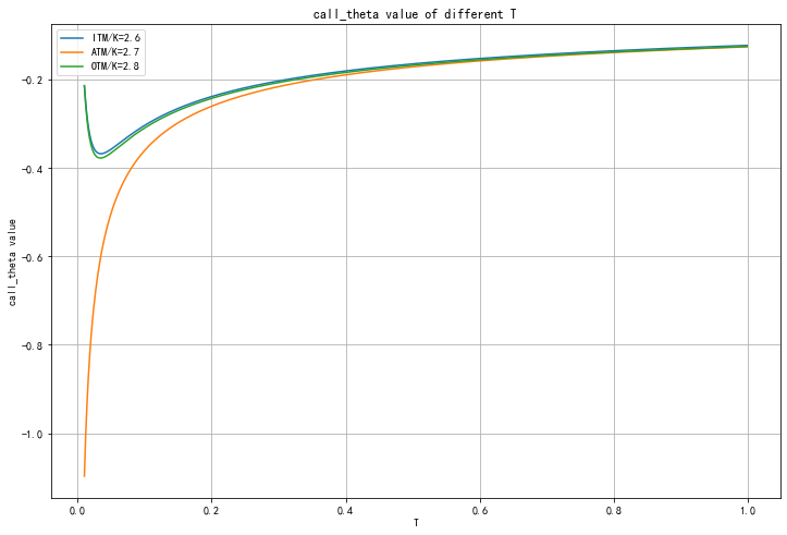
It can be seen from the figure that the shorter the remaining period, the faster the time decay, Θ\ Theta Θ The more negative, compared with real and imaginary options, the parity option theta has the largest negative value. The faster the maturity, the higher the sensitivity of the average value

two Θ Relationship between put and T

# # 
K1=2.6
K2=2.5
K3=2.4
St=2.5
T = np.arange(0.01, 1, 0.001)
pput_theta=[put_theta(St, K1, t, T, r, sigma) for T in T]
pput_theta_1=[put_theta(St, K2, t, T, r, sigma) for T in T]
pput_theta_2=[put_theta(St, K3, t, T, r, sigma) for T in T]

# # Put option
plt.figure(figsize=(12, 8))

plt.xlabel('T')
plt.ylabel("put_theta value")
plt.title('put_theta value of different T')

plt.plot(T, pput_theta,label='OTM/K=2.6')
plt.plot(T, pput_theta_1,label='ATM/K=2.5')
plt.plot(T, pput_theta_2,label='ITM/K=2.4')
plt.grid()
plt.legend()

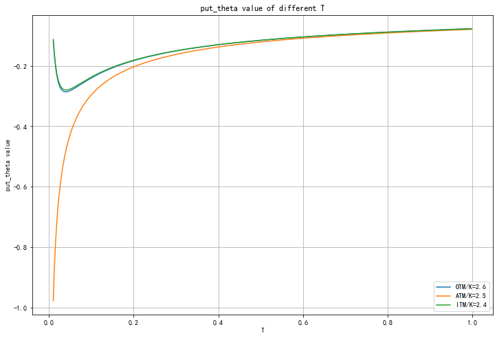
For put option, the relationship between theta and T is basically the same as that of call option.

IV Θ Relationship with St and T

Next, modeling. Describe the relationship between theta and the underlying asset price and maturity days.

one Θ Relationship between call and St, T

def plot_greeks(function, greek):
    # parameter
    St =2.5  # 50ETF value
    
    t = 0.0  # valuation date
    
    r = 0.015  # risk-less short rate
    sigma = 0.2  # volatility

    # Calculate the green of options
    tlist = np.linspace(0.01, 1, 25)
    klist = np.linspace(2.2, 2.9, 25)
    V = np.zeros((len(tlist), len(klist)), dtype=np.float)
    for j in range(len(klist)):
        for i in range(len(tlist)):
            V[i, j] = function(St, klist[j], t, tlist[i], r, sigma)

    # 3D Plotting
    x, y = np.meshgrid(klist, tlist)
    fig = plt.figure(figsize=(9, 5))
    plot = p3.Axes3D(fig)
    plot.plot_surface(x, y, V,cmap='rainbow')
    plot.set_xlabel('strike $K$')
    plot.set_ylabel('maturity $T$')
    plot.set_zlabel('%s(K, T)' % greek)

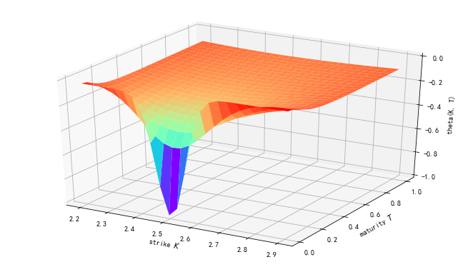
two Θ Relationship between put and St, T

plot_greeks(put_theta, 'theta')

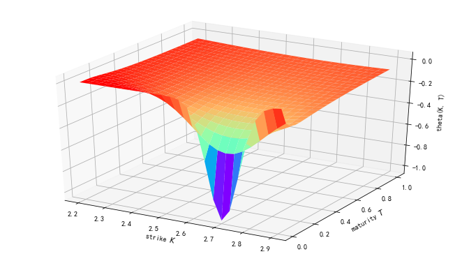
As can be seen from the figure, theta is the smallest near short-term parity options. With the passage of time, theta of parity options increases( Θ) Will gradually increase.

summary

Theta value reflects the value lost by option buyers over time, so theta value is still an important sensitivity index.