Super parameter optimization methods: grid search, random search, Bayesian Optimization (BO) and other algorithms.
reference material: Three super parameter optimization methods are explained in detail, as well as code implementation
Experimental basic code
import numpy as np
import pandas as pd
from lightgbm.sklearn import LGBMRegressor
from sklearn.metrics import mean_squared_error
import warnings

warnings.filterwarnings('ignore')
from sklearn.datasets import load_diabetes
from sklearn.model_selection import KFold, cross_val_score
from sklearn.model_selection import train_test_split
import timeit
import os
import psutil

# In sklearn Datasets's diabetes dataset demonstrates and compares different algorithms to load it.
diabetes = load_diabetes()
data = diabetes.data
targets = diabetes.target
n = data.shape[0]
random_state = 42
# Time occupation s
start = timeit.default_timer()
# Memory usage mb
info_start = psutil.Process(os.getpid()).memory_info().rss / 1024 / 1024
train_data, test_data, train_targets, test_targets = train_test_split(data, targets,
                                                                      test_size=0.20, shuffle=True,
                                                                      random_state=random_state)
num_folds = 2
kf = KFold(n_splits=num_folds, random_state=random_state, shuffle=True)
model = LGBMRegressor(random_state=random_state)
score = -cross_val_score(model, train_data, train_targets, cv=kf, scoring="neg_mean_squared_error", n_jobs=-1).mean()
print('score: ', score)

end = timeit.default_timer()
info_end = psutil.Process(os.getpid()).memory_info().rss / 1024 / 1024

print('This program takes up memory' + str(info_end - info_start) + 'mB')
print('Running time:%.5fs' % (end - start))
The experimental results are as follows:
Least square error: 3897.5550693355276
This program takes up 0.5mB of memory
Running time:1.48060s
For comparison purposes, we will optimize the model that only adjusts the following three parameters:
n_estimators: from 100 to 2000
max_depth: 2 to 20
learning_rate: from 10e-5 to 1
1, Grid search
Grid search is probably the simplest and most widely used hyperparametric search algorithm. It determines the optimal value by finding all points in the search range. If a larger search range and a smaller step size are used, the grid search has a high probability of finding the global optimal value. However, this search scheme consumes a lot of computing resources and time, especially when there are many super parameters to be tuned.
Therefore, in the process of practical application, the grid search method generally uses a wider search range and larger step size to find the possible location of the global optimal value; Then narrow the search range and step size to find a more accurate optimal value. This operation scheme can reduce the time and computation required, but because the objective function is generally non convex, it is likely to miss the global optimal value.
The grid search element corresponds to the element in sklearn GridSearchCV Module: sklearn model_ selection. GridSearchCV
(estimator, param_grid, , scoring=None, n_jobs=None, iid='deprecated', refit=True, cv=None, verbose=0, pre_dispatch='2n_jobs', error_score=nan, return_train_score=False). See blog for details.
1.1 GridSearch algorithm code
from sklearn.model_selection import GridSearchCV
# Time occupation s
start = timeit.default_timer()
# Memory usage mb
info_start = psutil.Process(os.getpid()).memory_info().rss / 1024 / 1024

param_grid = {'learning_rate': np.logspace(-3, -1, 3),
              'max_depth': np.linspace(5, 12, 8, dtype=int),
              'n_estimators': np.linspace(800, 1200, 5, dtype=int),
              'random_state': [random_state]}
gs = GridSearchCV(model, param_grid, scoring='neg_mean_squared_error',
                  n_jobs=-1, cv=kf, verbose=False)
gs.fit(train_data, train_targets)
gs_test_score = mean_squared_error(test_targets, gs.predict(test_data))

end = timeit.default_timer()
info_end = psutil.Process(os.getpid()).memory_info().rss / 1024 / 1024

print('This program takes up memory' + str(info_end - info_start) + 'mB')
print('Running time:%.5fs' % (end - start))
print("Best MSE {:.3f} params {}".format(-gs.best_score_, gs.best_params_))
Experimental results:
This program takes up 12.79296875mB of memory
Running time:6.35033s
Best MSE 3696.133 params {'learning_rate': 0.01, 'max_depth': 5, 'n_estimators': 800, 'random_state': 42}
1.2 visual interpretation
import matplotlib.pyplot as plt
gs_results_df = pd.DataFrame(np.transpose([-gs.cv_results_['mean_test_score'],
                                           gs.cv_results_['param_learning_rate'].data,
                                           gs.cv_results_['param_max_depth'].data,
                                           gs.cv_results_['param_n_estimators'].data]),
                             columns=['score', 'learning_rate', 'max_depth',
                                      'n_estimators'])
gs_results_df.plot(subplots=True, figsize=(10, 10))
plt.show()
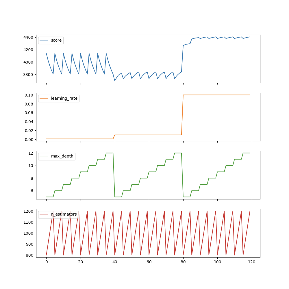
We can see, for example, max_depth is the least important parameter and it will not significantly affect the score. However, we are searching for max_ Eight different values of depth, and any fixed value is searched on other parameters. Obviously a waste of time and resources.
2, Random search
https://www.cnblogs.com/cgmcoding/p/13634531.html
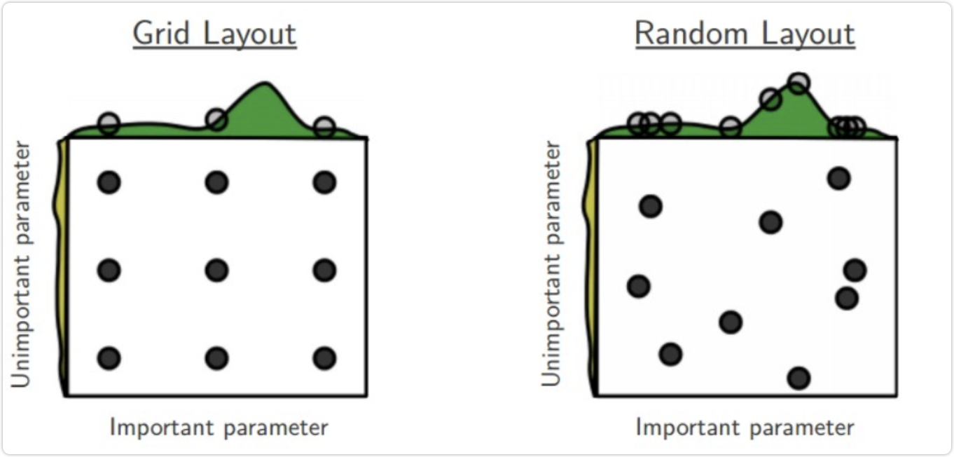
The idea of random search is similar to network search, except that all values between the upper and lower bounds are no longer tested, but sample points are randomly selected within the search range. His theoretical basis is that if the sample point set is large enough, the global optimal value or approximate value can be roughly found through random sampling. Random search is generally faster than web search. When searching for super parameters, if the number of super parameters is small (three or four or less), we can use grid search, an exhaustive search method. However, when the number of super parameters is large, we still use grid search, and the search time will increase exponentially.
Therefore, someone proposed a random search method, which randomly searches hundreds of points in the hyperparametric space, among which there may be relatively small values. This method is faster than the above sparse grid method, and experiments show that the random search method is slightly better than the sparse grid method. RandomizedSearchCV uses a method similar to the GridSearchCV class, but instead of trying all possible combinations, it selects a specific number of random combinations of a random value of each super parameter. This method has two advantages:
If you run a random search, say 1000 times, it will explore 1000 different values of each super parameter (instead of just a few values of each super parameter, as in grid search)
You can easily control the calculation amount of super parameter search by setting the search times.
The use method of randomized searchcv is actually the same as that of GridSearchCV, but it replaces GridSearchCV's grid search for parameters by sampling randomly in the parameter space. For parameters with continuous variables, randomized searchcv will sample them as a distribution, which is impossible for grid search, and its search ability depends on the set n_iter parameter, the same code is given.
Random search for sklearn in sklearn model_ selection. RandomizedSearchCV
(estimator, param_distributions, *, n_iter = 10, score = None, n_jobs = None, iid = 'deprecated', refine = true, cv = None, verbose = 0, pre_dispatch = '2 * n_jobs', random_state = None, error_score = nan, _return_train_score = False) The parameters are roughly the same as GridSearchCV, but there is an additional n_ ITER is the number of iteration rounds.
from sklearn.model_selection import RandomizedSearchCV
from scipy.stats import randint

param_grid_rand = {'learning_rate': np.logspace(-5, 0, 100),
                   'max_depth': randint(2, 20),
                   'n_estimators': randint(100, 2000),
                   'random_state': [random_state]}
# Time occupation s
start = timeit.default_timer()
# Memory usage mb
info_start = psutil.Process(os.getpid()).memory_info().rss / 1024 / 1024
rs = RandomizedSearchCV(model, param_grid_rand, n_iter=50, scoring='neg_mean_squared_error',
                        n_jobs=-1, cv=kf, verbose=False, random_state=random_state)

rs.fit(train_data, train_targets)

rs_test_score = mean_squared_error(test_targets, rs.predict(test_data))
end = timeit.default_timer()
info_end = psutil.Process(os.getpid()).memory_info().rss / 1024 / 1024

print('This program takes up memory' + str(info_end - info_start) + 'mB')
print('Running time:%.5fs' % (end - start))
print("Best MSE {:.3f} params {}".format(-rs.best_score_, rs.best_params_))
This program takes up 17.90625mB of memory
Running time:3.85010s
Best MSE 3516.383 params {'learning_rate': 0.0047508101621027985, 'max_depth': 19, 'n_estimators': 829, 'random_state': 42}
It can be seen that the effect is better than that of GridSearchCV when running 50 rounds, and the time is shorter.
3, Bayesian Optimization (BO)
  Grid search is slow, but it works well in searching the whole search space, while random search is fast, but it may miss important points in the search space. Fortunately, there is a third option: Bayesian optimization. In this paper, we will focus on an implementation of Bayesian Optimization called hyperopt of Python modular. Bayesian optimization algorithm is used to find the optimal and maximum parameters. It adopts a completely different method from grid search and random search. When testing a new point, grid search and random search will ignore the information of the previous point, while Bayesian optimization algorithm makes full use of the previous information. Bayesian optimization algorithm learns the shape of the objective function and finds the parameters that improve the objective function to the global optimal value.
  Specifically, the method of learning objective function is to assume a search function according to a priori distribution; Then, every time a new sampling point is used to test the objective function, this information is used to update the prior distribution of the objective function; Finally, the algorithm tests the points where the global maximum value given by the a posteriori distribution may appear. For Bayesian optimization algorithm, one thing to note is that once a local optimal value is found, it will continuously sample in the region, so it is easy to fall into the local optimal value. In order to make up for this shortcoming, Bayesian algorithm will find a balance between exploration and utilization. Exploration is to obtain sampling points in the area that has not been sampled, while utilization will sample in the most likely global maximum area according to the posterior distribution.
  We will use[hyperopt library](http://hyperopt.github.io/hyperopt/#documentation) to handle this algorithm. It is one of the most popular libraries for hyperparametric optimization. See the blog for details.
(1)TPE algorithm:
algo=tpe.suggest
TPE is the default algorithm for Hyperopt. It uses Bayesian method for optimization. At each step, it tries to establish the probability model of the function and select the most promising parameters for the next step. This kind of algorithm works as follows:
- Generate random initial point x
- Calculate F(x)
- Try to establish conditional probability model P(F|x) by using test history
- Selecting xi according to P(F|x) is most likely to lead to better F(xi)
- Calculate the actual value of F(xi)
- Repeat steps 3-5 until one of the stop conditions is met, such as I > max_ evals
from hyperopt import fmin, tpe, hp, anneal, Trials
def gb_mse_cv(params, random_state=random_state, cv=kf, X=train_data, y=train_targets):
    # the function gets a set of variable parameters in "param"
    params = {'n_estimators': int(params['n_estimators']),
              'max_depth': int(params['max_depth']),
             'learning_rate': params['learning_rate']}

    # we use this params to create a new LGBM Regressor
    model = LGBMRegressor(random_state=random_state, **params)

    # and then conduct the cross validation with the same folds as before
    score = -cross_val_score(model, X, y, cv=cv, scoring="neg_mean_squared_error", n_jobs=-1).mean()

    return score
# State space, minimize the value range of params of the function
space={'n_estimators': hp.quniform('n_estimators', 100, 2000, 1),
       'max_depth' : hp.quniform('max_depth', 2, 20, 1),
       'learning_rate': hp.loguniform('learning_rate', -5, 0)
      }

# trials will record some information
trials = Trials()
#Time occupation s
start=timeit.default_timer()
#Memory usage mb
info_start = psutil.Process(os.getpid()).memory_info().rss/1024/1024
best=fmin(fn=gb_mse_cv, # function to optimize
          space=space,
          algo=tpe.suggest, # optimization algorithm, hyperotp will select its parameters automatically
          max_evals=50, # maximum number of iterations
          trials=trials, # logging
          rstate=np.random.RandomState(random_state) # fixing random state for the reproducibility
         )

# computing the score on the test set
model = LGBMRegressor(random_state=random_state, n_estimators=int(best['n_estimators']),
                      max_depth=int(best['max_depth']),learning_rate=best['learning_rate'])
model.fit(train_data,train_targets)
tpe_test_score=mean_squared_error(test_targets, model.predict(test_data))
end=timeit.default_timer()
info_end = psutil.Process(os.getpid()).memory_info().rss/1024/1024

print('This program takes up memory'+str(info_end-info_start)+'mB')
print('Running time:%.5fs'%(end-start))
print("Best MSE {:.3f} params {}".format( gb_mse_cv(best), best))
Experimental results:
This program takes up 2.5859375mB of memory
Running time:52.73683s
Best MSE 3186.791 params {'learning_rate': 0.026975706032324936, 'max_depth': 20.0, 'n_estimators': 168.0}
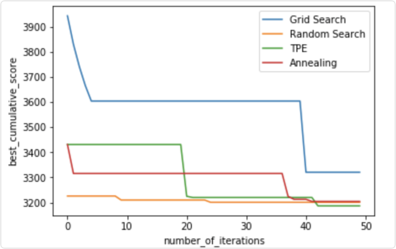
4, Conclusion
We can see that even in the next steps, TPE and annealing algorithm will actually improve the search results over time, while random search randomly found a good solution at the beginning, and then only slightly improved the results. The current difference between TPE and RandomizedSearch results is small, but hyperopt can significantly improve time / score in some real-world applications with a more diversified range of super parameters