Starting from 0, data analysis and machine learning in Xueda University are simple and simple to write down the contest experience. This paper uses a variety of machine learning regression algorithms, and also uses deep learning pytorch to build a neural network for regression calculation.

1. Background introduction

This is an industrial steam volume contest, linked: AI Training Camp Computer Vision-Ali Yuntianchi

Contest Background

The basic principle of fossil fuel power generation is that fuel heats up water to produce steam while burning, steam pressure drives the steam turbine to rotate, and then the steam turbine drives the generator to rotate to generate electricity. In this series of energy conversion, the core affecting the power generation efficiency is the boiler's combustion efficiency, that is, the fuel burns the heated water to produce high temperature and high pressure steam.Includes the boiler's adjustable parameters, such as combustion feed, primary and secondary air, induced air, return air, water supply; and the boiler's operation, such as the boiler bed temperature, bed pressure, furnace temperature, pressure, superheater temperature and so on.

Description of the title

The data collected by the desensitization boiler sensor (acquisition frequency is at the level of minutes) can be used to predict the amount of steam generated according to the boiler's operation.

2. Data Exploration

Download the training and test sets locally, open jupyter notebook, and import the packages.

import numpy as np
import pandas as pd
import matplotlib.pyplot as plt
import seaborn as sns
from scipy import stats

import warnings
warnings.filterwarnings("ignore")
%matplotlib inline

Start importing data.

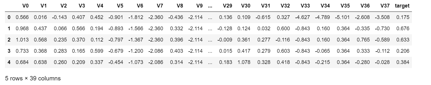
train_data_file = "data/zhengqi_train.txt"
test_data_file = "data/zhengqi_test.txt"

train_data = pd.read_csv(train_data_file, sep="\t", encoding="utf-8")
test_data = pd.read_csv(test_data_file, sep="\t", encoding="utf-8")

#View the first few rows of data
train_data.head()

The data for train_data is as follows:

View the basic information of the training set as follows:

train_data.info()

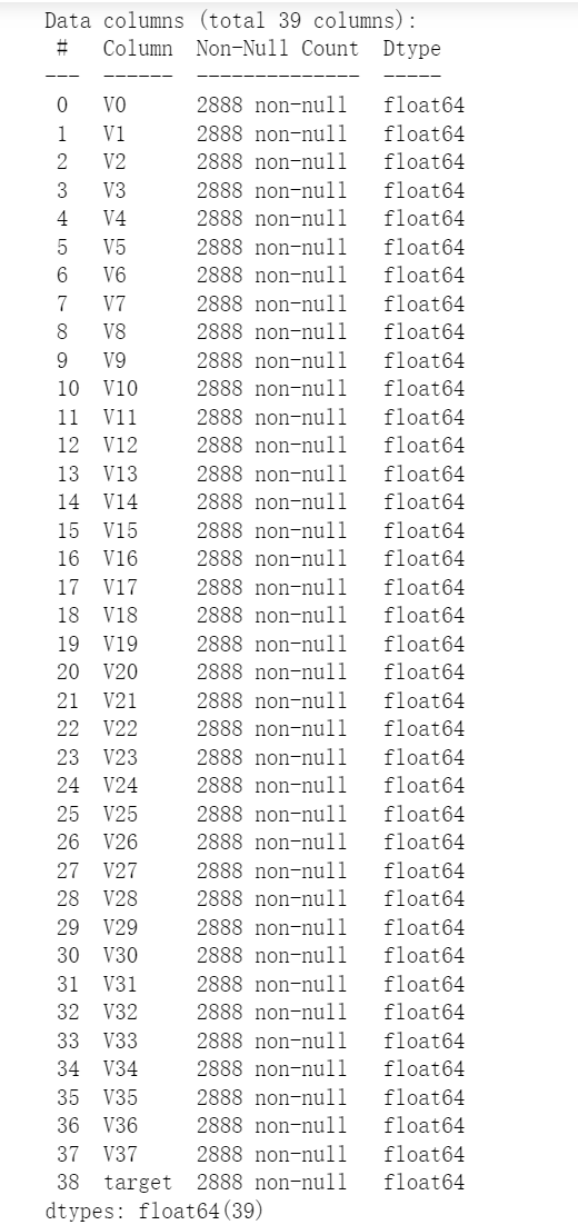
You can see that:

1. A total of 2888 data, numbered 0-2887
2. A total of 39 columns, excluding the result column, with 38 eigenvectors
3. All columns have no missing values and are of numeric type

 

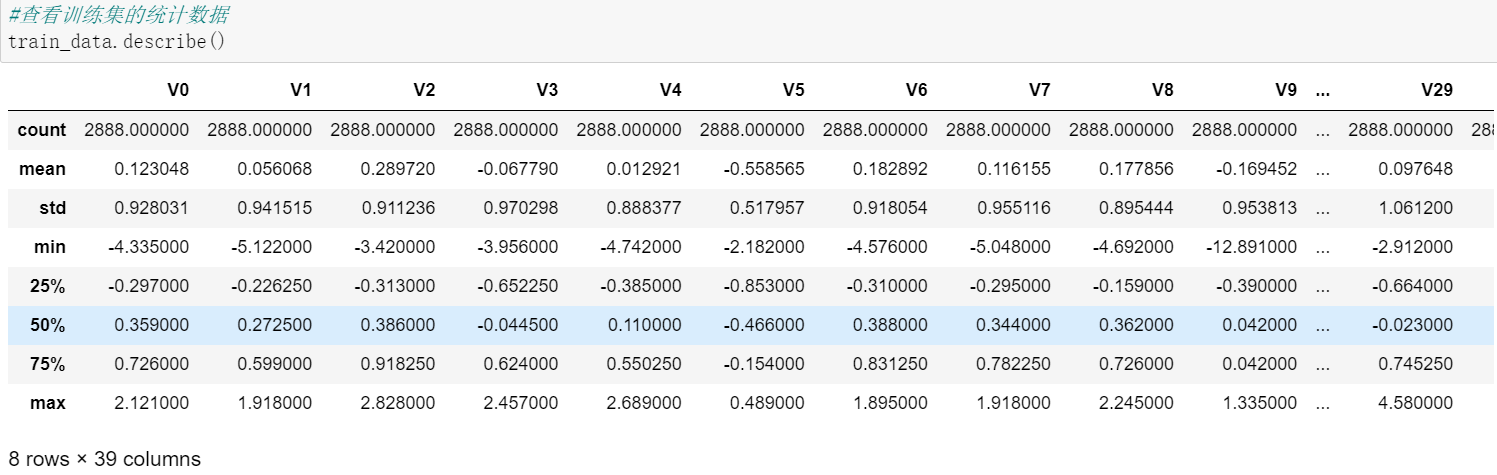
Call the describe() method again to view the information of the training set:

Data visualization

In order to visualize the relationship between data more intuitively, data visualization is required.

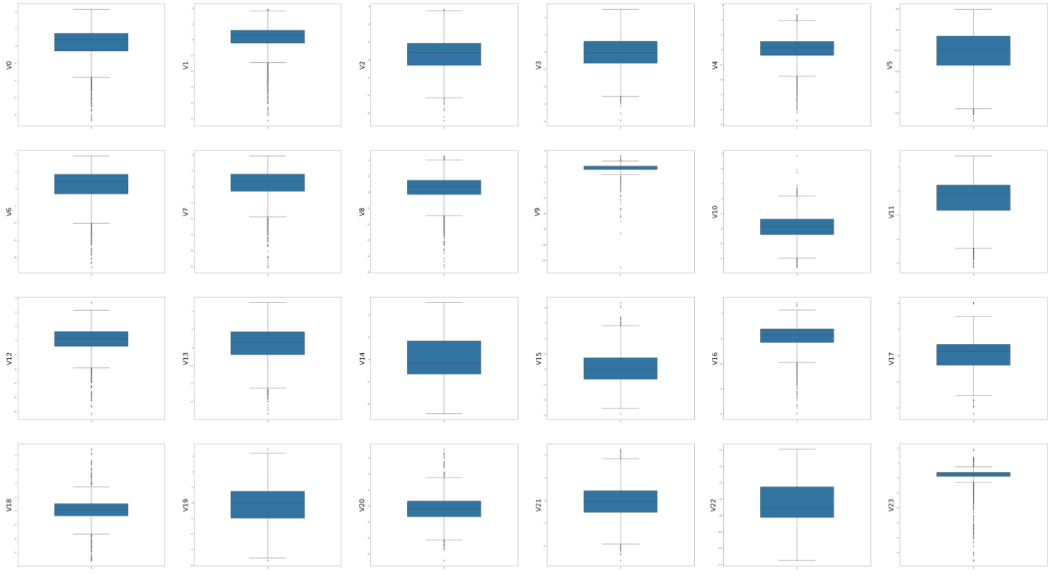
First, plot box charts of each feature:

column_list = train_data.columns.tolist()[:39]                                #List Header List
fig = plt.figure(figsize=(100, 100), dpi=75)                                  #Specify the width and height of the drawing object
for i in range(38):
    plt.subplot(7, 6, i+1)                                                    #7 Rows 8 Columns Subgraph
    sns.boxplot(data=train_data[column_list[i]], orient="v", width=0.5)
    plt.ylabel(column_list[i], fontsize=36)
plt.show()

The results are as follows:

 

Draw histograms and Q-Q charts of each feature. Q-Q charts are used to describe whether data conforms to a normal distribution. If points fall on a straight line, the data conforms to a standard normal distribution.

#Draw histograms and Q-Q graphs of all variables
train_cols = 6
train_rows = len(train_data.columns)
plt.figure(figsize=(4*train_cols, 4*train_rows))

i = 0
for col in train_data.columns:
    i += 1
    ax = plt.subplot(train_rows, train_cols, i)
    sns.distplot(train_data[col], fit=stats.norm)
    
    i += 1
    ax = plt.subplot(train_rows, train_cols, i)
    res = stats.probplot(train_data[col], plot=plt)
    
plt.tight_layout()                                                 #tight_layout automatically adjusts the subgraph parameters to fill the entire image area
plt.show()

The effect is as follows:

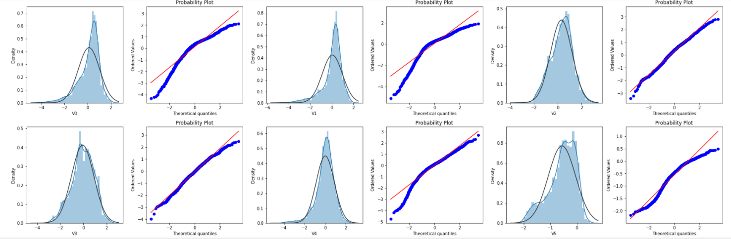
Due to space limitation, only part of the picture is shown here.

The KDE diagram of each feature is drawn to show whether the distribution of training set and test set data is consistent. If the distribution of training set data is not consistent with that of test set data, it indicates that there are some problems with this feature and it needs to be excluded when doing model training.

train_cols = 6
train_rows = len(test_data.columns)
plt.figure(figsize=(4*train_cols, 4*train_rows))

for i in range(train_rows):
    ax = plt.subplot(train_rows, train_cols, i+1)
    ax = sns.kdeplot(train_data[column_list[i]], color="Red", shade=True)
    ax = sns.kdeplot(test_data[column_list[i]], color="Blue", shade=True)
    ax.set_xlabel(column_list[i])
    ax.set_ylabel("Frequency")
    ax = ax.legend(["train", "test"])                                             #Legend
plt.show()

The effect is as follows:

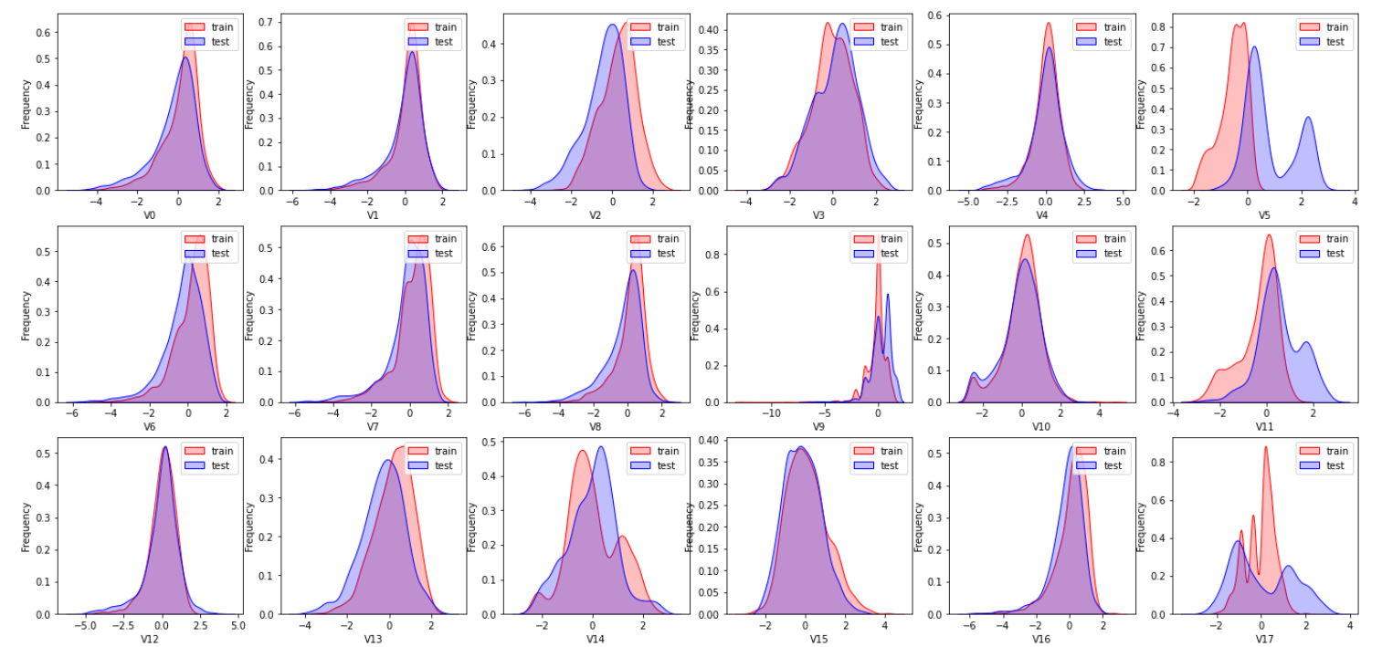
Due to space limitation, only part of the graph is shown here. From the graph, we can see that the distribution of the feature variables v5, v9, v11, v17, v22, v28 in the training set and the test set are inconsistent, such features need to be deleted in the training model.

Next, we calculate the correlation coefficients for each feature.

data_train1 = train_data.drop(["V5", "V9", "V11", "V17", "V22", "V28"], axis=1)
train_corr = data_train1.corr()
train_corr

The effect is as follows:

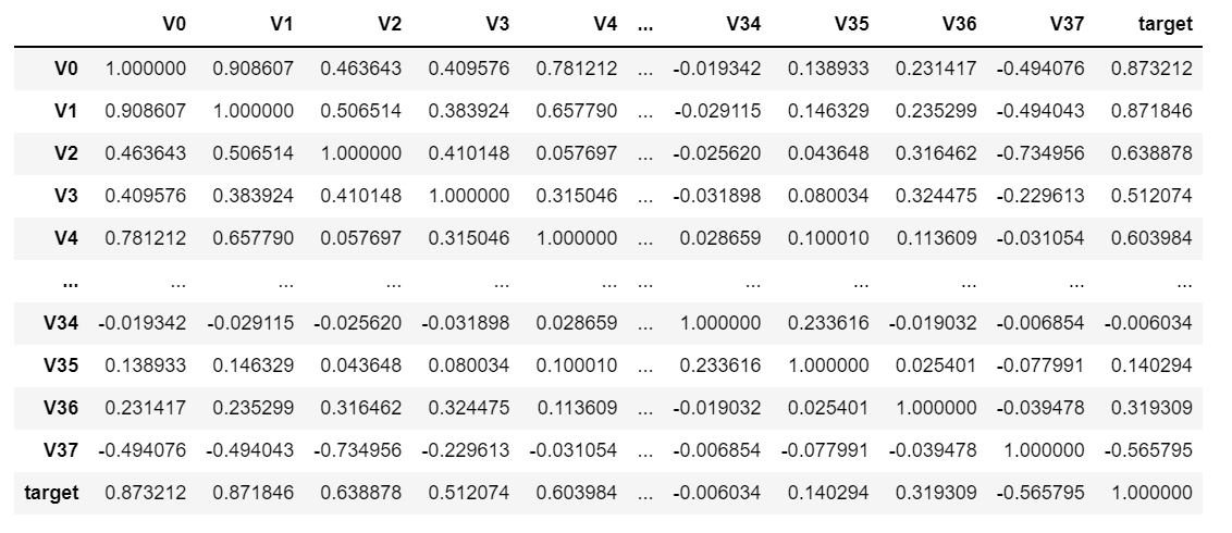
It looks like it's hard to see something. What do you do? Data visualization is certainly used to make icons:

ax = plt.subplots(figsize=(20, 16))                                 #Canvas Size
ax = sns.heatmap(train_corr, vmax=0.8, square=True, annot=True)     #Draw thermogram

The effect is as follows:

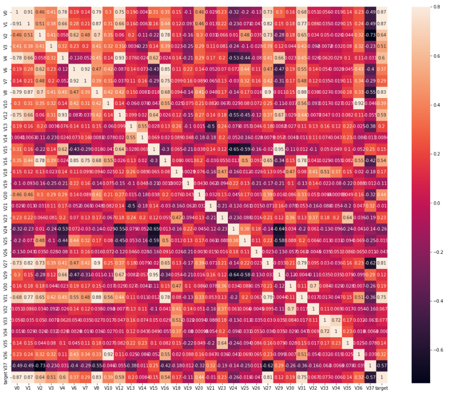
How about this? Plus, does the graph feel much better, but it still has a lot of data, so it's impossible to visually see the information you want. Don't worry, we can find 10 most relevant characteristic variables to the target variable to further reduce the amount of data.

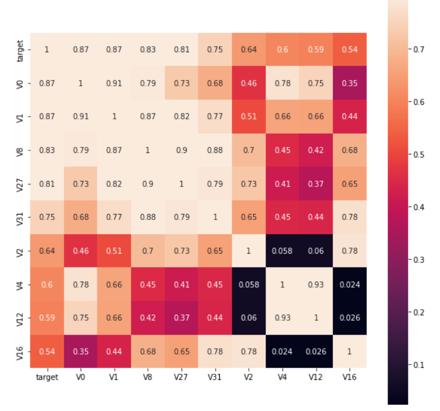
k = 10                                                                               #Find k the k most relevant characteristic variables to the target variable
cols = train_corr.nlargest(k, "target")["target"].index                              #index of k most relevant columns

#cm = np.corrcoef(train_data[cols].values.T)
hm = plt.subplots(figsize=(10, 10))                                                  #Canvas Size
hm = sns.heatmap(train_data[cols].corr(), vmax=0.8, square=True, annot=True)        #Draw thermogram
plt.show()

The effect is as follows:

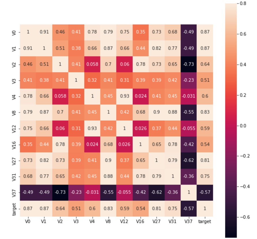
Or we can also find features with correlation coefficients greater than 0.5:

rate = 0.5
top_corr_features = train_corr.index[abs(train_corr["target"]) > rate]
plt.figure(figsize=(10, 10))
hm = sns.heatmap(train_data[top_corr_features].corr(), vmax=0.8, square=True, annot=True)        #Draw thermogram

The effect is as follows:

3. Modeling

Write how to use deep learning pytorch to build a neural network for regression prediction.

First, import the package:

import pandas as pd
import torch
from torch import nn
from sklearn import preprocessing
import torch.optim as optim
import random
from sklearn.decomposition import PCA

Read data:

#Read data
#Description: No missing values for data
train_data_file = "data/zhengqi_train.txt"
test_data_file = "data/zhengqi_test.txt"
#read
train_data = pd.read_csv(train_data_file, sep="\t", encoding="utf-8")
test_data = pd.read_csv(test_data_file, sep="\t", encoding="utf-8")

After importing the data, we need to normalize the data, so it is more convenient to combine the training set and the test set first. After normalization, we can split the data.

#Merge training and test sets
all_features = pd.concat((train_data.iloc[:,0:-1], test_data.iloc[:,0:]))

#data normalization
features_columns = all_features.dtypes[all_features.dtypes != "object"].index                   #column
#Normalization function
min_max_scaler = preprocessing.MinMaxScaler()
min_max_scaler = min_max_scaler.fit(all_features[features_columns])
#Start processing
all_features_scaler = min_max_scaler.transform(all_features[features_columns])
all_features_scaler = pd.DataFrame(all_features_scaler)
all_features_scaler.columns = features_columns
#Split data
n_train = train_data.shape[0]
train_features = torch.tensor(all_features[:n_train].values, dtype=torch.float32)
test_features = torch.tensor(all_features[n_train:].values, dtype=torch.float32)
train_labels = torch.tensor(train_data.target.values.reshape(-1, 1), dtype=torch.float32)

Simply do a feature project, mainly using principal component analysis:

#PCA processing for feature dimension reduction
pca = PCA(n_components=16)
train_features_16 = pca.fit_transform(train_features)
test_features_16 = pca.transform(test_features)
train_features_16 = torch.tensor(train_features_16, dtype=torch.float32)
test_features_16 = torch.tensor(test_features_16, dtype=torch.float32)

Then slice the dataset so that we can evaluate the model.

#Fractional dataset
from sklearn.model_selection import train_test_split        #Fractional data

#Divide dataset, 80% training set, 20% test set
train_data, test_data, train_target, test_target = train_test_split(train_features_16, train_labels, test_size=0.2, random_state=0)

Now it is time to define our neural network:

#Define Neural Network
class MyNet(nn.Module):
    def __init__(self, in_features, out_features=1):
        super().__init__()
        self.fc = nn.Sequential(
            nn.Linear(in_features, 12),
            nn.GELU(),
            nn.Linear(12, 10),
            nn.GELU(),
            nn.Linear(10, out_features),
        )

    def forward(self, x):
        return self.fc(x)

With a handwritten neural network, simply use the three linear regression layers, because it is a regression problem, so the output of the neural network is only 1, where the activation function is gelu, Gelu effect is better than relu.

When running a neural network, GPU runs much faster than CPU if conditions permit.

device = torch.device("cuda")
in_features = train_features_16.shape[1]
#print(in_features)
net = MyNet(in_features).to(device)
loss = nn.MSELoss()
optimizer = optim.Adam(net.parameters(), lr=0.001)

train_net = True
if train_net:
    for epoch in range(230):
        #net.train()
        for X, y in data_iter(train_data, train_target, 210):
            X = X.to(device)
            y = y.to(device)
            X_out = net(X)
            l = loss(X_out, y)

            optimizer.zero_grad()
            l.backward()
            optimizer.step()

        print("epoch: ",epoch, "train_loss: ",l.item())

    #torch.save(net.state_dict(), 'model/model.pth')

Then try the network with a sliced set of validations:

#Validation Set Loss
test_data = test_data.to(device)
test_target = test_target.to(device)
predict = net(test_data)
l = loss(predict, test_target)
print("the loss: ", l)

Next, just hand in the results:

Ouch, I'm still a chicken and I'm crying.