Time series analysis - 23 DTW (time series similarity measurement algorithm)
Preliminary study on DTW
brief introduction
In time series analysis, DTW(Dynamic Time Warping) is an algorithm used to detect the similarity of two time series, which is usually represented by a distance. For example, the following two sequences,
a
=
[
1
,
2
,
3
]
a=[1,2,3]
a=[1,2,3]
b
=
[
3
,
2
,
2
]
b=[3,2,2]
b=[3,2,2]
How do we measure the distance between the two sequences? An obvious method is to calculate the distance of the elements in the two sequences one by one according to their positions, and finally add it up or average it after adding it up. It sounds like a relatively simple and easy to understand method. We can observe the following figure to understand the measurement of temporal similarity.
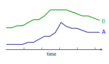
But if it's the following sequence,
a
=
[
1
,
2
,
3
]
a=[1,2,3]
a=[1,2,3]
b
=
[
2
,
2
,
2
,
3
,
4
]
b=[2,2,2,3,4]
b=[2,2,2,3,4]
What should we do?
DTW is one of the most commonly used algorithms to solve such problems.
In fact, this algorithm can not solve the problem that the length of the two sequences is not the same, even if the length of the sequence is not the same.
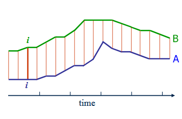
In short, DTW algorithm provides the elastic alignment of two sequences, finds the best alignment, and calculates the distance based on the best alignment.
application
DTW has a very wide range of applications. For example, it can be used to find similar walking patterns, even if one is walking fast, the other is walking slowly, or one is decelerating or accelerating.

DTW has been applied to a variety of serializable data such as video, audio and image, such as identifying speakers according to audio, signature recognition and so on.
Another typical application is in the time series analysis of the stock market. In the stock market, people always hope to predict the future, but the general machine learning algorithm is not very effective in this field. Because the prediction task of machine learning generally requires that its training set and test set have the same dimensional feature attributes. But we know that even if the very same pattern of a stock appears, the reflection length of their K-line and other indicators is not the same.
DTW algorithm rules
DTW is to calculate the optimal matching of two sequences under certain rules and constraints:
- Each location element of the first sequence must match one or more location elements of the second sequence, and vice versa.
- The first element of the first sequence must match the first element of the second sequence, but it can also match other locations.
- The last element of the first sequence must match the last element of the second sequence, but it can also match other locations.
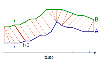
- The position mapping relationship between two sequences must be monotonically increasing, and vice versa. For example, if the 1,3 position of the first sequence is mapped to the 2,3 position of the second sequence, it is OK, but if it is mapped to the 3,2 position, it is not possible.
Optimal matching is the matching with minimum loss under all the above constraints. The minimum loss is the sum of the distances of the values on the mapping position. To sum up, the head and tail must match. There is no cross mapping and no residue subsequence.
Let's look at the pseudo code first:
int DTWDistance( s: array [1..n],  t: array [1..m] ) {
    DTW := array [0..n, 0..m]

    for i := 0 to n
        for j := 0 to m
            DTW[i, j] := infinity
    DTW[0, 0] := 0

    for i := 1 to n
        for j := 1 to m
            cost := d(s[i], t[j])
            DTW[i, j] := cost + minimum(DTW[i-1, j  ],    // insertion
                                        DTW[i  , j-1],    // deletion
                                        DTW[i-1, j-1])    // match

    return DTW[n, m]
}
here,
d
(
x
,
y
)
=
∣
x
−
y
∣
d(x,y)=|x-y|
d(x,y) = ∣ x − y ∣ and
D
T
W
[
i
,
j
]
DTW[i,j]
DTW[i,j] represents the sequence under the best alignment
s
[
1
:
i
]
s[1:i]
s[1:i] and
t
[
1
:
j
]
t[1:j]
Distance between t[1:j].
The core of this algorithm is:
DTW[i, j] := cost + minimum(DTW[i-1, j ], //insertion
                   DTW[i  , j-1],  //deletion
                   DTW[i-1, j-1])  //match
Obviously, this is a dynamic programming algorithm. Two sequences s [ 1 : i ] s[1:i] s[1:i] and t [ 1 : j ] t[1:j] The distance between t[1:j] is i i i and j j The distance of j plus the minimum distance of the following three subproblems
- Sub question 1: DTW[i-1,j] is understood as s s s sequence inserts a point
- Sub question 2: DTW[i,j-1] is understood as t t t sequence deletes a point
- Sub problem 3: DTW[i-1,j-1] is understood as two sequences matching at the last time point
Python code is as follows
def dtw(s, t):
    n, m = len(s), len(t)
    dtw_matrix = np.zeros((n+1, m+1))
    for i in range(n+1):
        for j in range(m+1):
            dtw_matrix[i, j] = np.inf
    dtw_matrix[0, 0] = 0

    for i in range(1, n+1):
        for j in range(1, m+1):
            cost = abs(s[i-1] - t[j-1])
            # take last min from a square box
            last_min = np.min([dtw_matrix[i-1, j], dtw_matrix[i, j-1], dtw_matrix[i-1, j-1]])
            dtw_matrix[i, j] = cost + last_min
    return dtw_matrix
for instance
import numpy as np
a = [1,2,3]
b = [2,2,2,3,4]
dtw(a,b)
array([[ 0., inf, inf, inf, inf, inf],
[inf, 1., 2., 3., 5., 8.],
[inf, 1., 1., 1., 2., 4.],
[inf, 2., 2., 2., 1., 2.]])
The value of the last element is the distance between the two sequences, which is 2.
Increase window limit
One problem with the above algorithm is that there is no limit to the number of elements that allow one element in one sequence to match another. In this case, if one of the sequences is too long, it will lead to performance problems. For example,
a
=
[
1
,
2
,
3
]
a=[1,2,3]
a=[1,2,3]
b
=
[
1
,
2
,
2
,
2
,
2
,
2
,
.
.
.
,
5
]
b=[1,2,2,2,2,2,...,5]
b=[1,2,2,2,2,2,...,5]
To avoid this problem, we can add a window parameter to limit the number of elements that one timing point can match in another timing point.
The pseudo code is as follows
int DTWDistance( s: array [1..n], t: array [1..m], w: int ) {

    DTW := array [0..n, 0..m]

    w := max(w, abs(n-m)) // adapt window size (*)

    for i := 0 to n
        for j:= 0 to m
            DTW[i, j] := infinity
    DTW[0, 0] := 0
    for i := 1 to n
        for j := max(1, i-w) to min(m, i+w)
            DTW[i, j] := 0

    for i := 1 to n
        for j := max(1, i-w) to min(m, i+w)
            cost := d(s[i], t[j])
            DTW[i, j] := cost + minimum(DTW[i-1, j  ],    // insertion
                               DTW[i  , j-1],    // deletion
                               DTW[i-1, j-1])    // match

    return DTW[n, m]
}
Python code is as follows
def dtw(s, t, window):
    n, m = len(s), len(t)
    w = np.max([window, abs(n-m)])
    dtw_matrix = np.zeros((n+1, m+1))

    for i in range(n+1):
        for j in range(m+1):
            dtw_matrix[i, j] = np.inf
    dtw_matrix[0, 0] = 0

    for i in range(1, n+1):
        for j in range(np.max([1, i-w]), np.min([m, i+w])+1):
            dtw_matrix[i, j] = 0

    for i in range(1, n+1):
        for j in range(np.max([1, i-w]), np.min([m, i+w])+1):
            cost = abs(s[i-1] - t[j-1])
            # take last min from a square box
            last_min = np.min([dtw_matrix[i-1, j], dtw_matrix[i, j-1], dtw_matrix[i-1, j-1]])
            dtw_matrix[i, j] = cost + last_min
    return dtw_matrix
a = [1,2,3,3,5]
b = [1,2,2,2,2,2,2,4]
dtw(a,b,window=3)
array([[ 0., inf, inf, inf, inf, inf, inf, inf, inf],
[inf, 0., 1., 2., 3., inf, inf, inf, inf],
[inf, 1., 0., 0., 0., 0., inf, inf, inf],
[inf, 3., 1., 1., 1., 1., 1., inf, inf],
[inf, 5., 2., 2., 2., 2., 2., 2., inf],
[inf, inf, 5., 5., 5., 5., 5., 5., 3.]])
Under the control of window parameters, the result is 3
Python package
The previous example code adopts recursion to realize dynamic planning. Although this method is simple to implement, its operation efficiency is very low. Therefore, in the actual scene, some optimization algorithms are generally used, such as
PrunedDTW, SparseDTW, FastDTW and MultiscaleDTW
Here we use FastDTW to audition
from fastdtw import fastdtw
from scipy.spatial.distance import euclidean

x = np.array([1, 2, 3, 3, 7])
y = np.array([1, 2, 2, 2, 2, 2, 2, 4])

distance, path = fastdtw(x, y, dist=euclidean)

print(distance)
print(path)

# 5.0
# [(0, 0), (1, 1), (1, 2), (1, 3), (1, 4), (2, 5), (3, 6), (4, 7)]
5.0
[(0, 0), (1, 1), (1, 2), (1, 3), (1, 4), (1, 5), (1, 6), (2, 7), (3, 7), (4, 7)]
Unfinished, to be continued