Time series analysis - missing value processing

This article is based on the article of Zhihu boss

Cleaning data

Data cleaning is an important part of data analysis, and time series data is no exception. This section will introduce the data cleaning methods for time series data in detail.

• Missing value processing
• Change time and frequency
• Smooth data
• Dealing with seasonal issues
• Prevent unconscious looking forward

Missing value processing

Missing values are common. For example, in a medical scenario, a time series data may be missing for the following reasons:

• The patient failed to comply with the doctor's advice
• The patient's health is very good, so it is not necessary to record it at every moment
• The patient was forgotten
• Random technical failure of medical equipment
• Data entry problem

The most commonly used methods to deal with missing values include imputation and deletion.

Imputation: filling missing values based on other values of the complete dataset

Deletion: directly delete the time period with missing value

Generally speaking, we prefer to retain data rather than delete it to avoid information loss. In the actual case, the way to take should consider whether it can bear the loss of deleting specific data.

This section will focus on three data filling methods and demonstrate how to use them in python:

• Forward fill
• Moving average
• Interpolation

The data set used is the annual unemployment rate data of the United States, and the data set is from OECD official website.

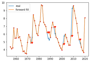
Forward fill

Forward filling method is one of the simplest methods to fill in data. The core idea is to fill in the current missing value with the value of the latest time point before the missing value. Using this method does not require any mathematics or complex logic.

Corresponding to forward filling, there is also a backward fill method. As the name suggests, it refers to filling with the value of the latest time point after the missing value. However, this method needs special caution because it is a lookahead behavior and can only be considered when you don't need to predict future data.

The advantages of forward filling method are summarized. It is simple to calculate and easy to be used for real-time streaming media data.

Moving average

Moving average method is another method to fill the data. The core idea is to take out the value in a rolling time before the missing value occurs, and calculate its average or median to fill the missing value. In some scenarios, this method will have better effect than forward filling. For example, the noise of data is very large and fluctuates greatly for a single data point, but the moving average method can weaken these noises.

Similarly, you can use the time point after the missing value occurs to calculate the mean value, but you need to pay attention to the lookahead problem.

Another small trick is that when calculating the mean, a variety of methods can be adopted according to the actual situation, such as exponential weighting, to give higher weight to the nearest data point.

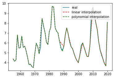
Interpolation

Interpolation is another method to determine the value of missing data points, which is mainly based on the constraints on various images we want the overall data to represent. For example, linear interpolation requires a certain linear fitting relationship between missing data and adjacent points. Therefore, interpolation is a priori method, and some business experience needs to be substituted when using interpolation.

In many cases, linear (or spline) interpolation is very suitable. For example, consider the average weekly temperature, where there is a known upward or upward trend, and the temperature drop depends on the time of the year. Or consider a growing business with known annual sales data. In these scenarios, the use of interpolation can achieve good results.

Of course, there are many situations that are not suitable for linear (or spline) interpolation. For example, in the absence of precipitation data in the weather data set, linear inference should not be made between known days, because the law of precipitation is not like this. Similarly, if we look at someone's sleep time every day, we should not use the linear extrapolation of sleep time of known days.

Python code implementation

import pandas as pd
import numpy as np
import matplotlib.pyplot as plt
%matplotlib inline
pd.set_option('max_row',1000)

# Import US annual unemployment rate data
unemploy = pd.read_csv('data\\unemployment.csv')

unemploy.head()

	year	rate
0	1955	4.383333
1	1956	4.141667
2	1957	4.258333
3	1958	6.800000
4	1959	5.475000

# Build a column of randomly missing values
unemploy['missing'] = unemploy['rate']
# Randomly select 10% rows and manually fill in the missing values
mis_index = unemploy.sample(frac=0.1,random_state=999).index
unemploy.loc[mis_index,'missing']=None

1. Use forward fill to fill in the missing value

unemploy['f_fill'] = unemploy['missing']
unemploy['f_fill'].ffill(inplace=True)

# Observe the filling effect
plt.scatter(unemploy.year,unemploy.rate,s=10)
plt.plot(unemploy.year,unemploy.rate,label='real')
plt.scatter(unemploy[~unemploy.index.isin(mis_index)].year,unemploy[~unemploy.index.isin(mis_index)].f_fill,s=10,c='r')
plt.scatter(unemploy.loc[mis_index].year,unemploy.loc[mis_index].f_fill,s=50,c='r',marker='v')
plt.plot(unemploy.year,unemploy.f_fill,label='forward fill')
plt.legend()

2. Use moving average to fill in the missing value

unemploy['moveavg']=np.where(unemploy['missing'].isnull(),
                             unemploy['missing'].shift(1).rolling(3,min_periods=1).mean(),
                             unemploy['missing'])

# Observe the filling effect
plt.scatter(unemploy.year,unemploy.rate,s=10)
plt.plot(unemploy.year,unemploy.rate,label='real')
plt.scatter(unemploy[~unemploy.index.isin(mis_index)].year,unemploy[~unemploy.index.isin(mis_index)].f_fill,s=10,c='r')
plt.scatter(unemploy.loc[mis_index].year,unemploy.loc[mis_index].f_fill,s=50,c='r',marker='v')
plt.plot(unemploy.year,unemploy.f_fill,label='forward fill',c='r',linestyle = '--')
plt.scatter(unemploy[~unemploy.index.isin(mis_index)].year,unemploy[~unemploy.index.isin(mis_index)].moveavg,s=10,c='r')
plt.scatter(unemploy.loc[mis_index].year,unemploy.loc[mis_index].moveavg,s=50,c='g',marker='^')
plt.plot(unemploy.year,unemploy.moveavg,label='moving average',c='g',linestyle = '--')
plt.legend()

3. Use interpolation to fill in missing values

# Try linear interpolation and polynomial interpolation
unemploy['inter_lin']=unemploy['missing'].interpolate(method='linear')
unemploy['inter_poly']=unemploy['missing'].interpolate(method='polynomial', order=3)

# Observe the filling effect
plt.plot(unemploy.year,unemploy.rate,label='real')
plt.plot(unemploy.year,unemploy.inter_lin,label='linear interpolation',c='r',linestyle = '--')
plt.plot(unemploy.year,unemploy.inter_poly,label='polynomial interpolation',c='g',linestyle = '--')
plt.legend()

Change data set time and frequency

Usually, we will find that the time axes from different data sources often cannot correspond one by one. At this time, we need to change the time and frequency to clean the data. Since the frequency of actual measurement data cannot be changed, what we can do is to change the frequency of data collection, that is, up sampling and down sampling mentioned in this section.

Down sampling

Downsampling refers to reducing the frequency of data collection, that is, the way to extract subsets from the original data.

The following are some scenes used in downsampling:

• The original resolution of the data is unreasonable: for example, there is a data recording the outdoor temperature, and the time frequency is once per second. We all know that the temperature will not change significantly at the second level, and the measurement error of the second level temperature data will even be greater than the fluctuation of the data itself. Therefore, this data set has a lot of redundancy. In this case, it may be more reasonable to take data every n elements.
• Pay attention to the information of a specific season: if we are worried about seasonal fluctuations in some data, we can only select a season (or month) for analysis, for example, only select the data in January of each year for analysis.
• Data matching: for example, you have two time series data sets, one with lower frequency (annual data) and one with higher frequency (monthly data). In order to match the two data sets for the next analysis, you can combine the high-frequency data, such as calculating the annual mean or median, so as to obtain the data set with the same time axis.

Up sampling

To some extent, upsampling is a way to obtain higher frequency data out of thin air. What we should remember is that using upsampling only allows us to obtain more data labels without adding additional information.

The following are some scenes used for up sampling:

• Irregular time series: used to deal with the problem of irregular time axis in multi table Association.

  For example, there are now two data, one recording the time and amount of donation

amt	dt
99	2019-2-27
100	2019-3-2
5	2019-6-13
15	2019-8-1
11	2019-8-31
1200	2019-9-15

Another data records the time and code of public activities

identifier	dt
q4q42	2019-1-1
4299hj	2019-4-1
bbg2	2019-7-1

At this time, we need to merge the data of the two tables, label each donation, and record the latest public activity before each donation. This operation is called rolling join. The associated data results are as follows.

identifier	dt	amt
q4q42	99	2019-2-27
q4q42	100	2019-3-2
4299hj	5	2019-6-13
bbg2	15	2019-8-1
bbg2	11	2019-8-31
bbg2	1200	2019-9-15

• Data matching: similar to the down sampling scenario, for example, we have a monthly unemployment rate data, which needs to be converted into daily data in order to match with other data. If we assume that new jobs generally start on the first day of each month, we can deduce that the daily unemployment rate of this month is equal to the unemployment rate of that month.

Through the above cases, we find that even in a very clean data set, because it is necessary to compare data with different scales from different dimensions, it is often necessary to use up sampling and down sampling methods.

Smooth data

Data smoothing is also a common data cleaning technique. In order to tell a more understandable story, smoothing is often performed before data analysis. Data smoothing is usually to eliminate some extreme values or measurement errors. Even if some extreme values themselves are true, but do not reflect the potential data pattern, we will smooth them out.

When describing the concept of data smoothing, you need to introduce the following figure layer by layer.

weighted averaging, that is, moving average mentioned above, is also the simplest smoothing technology, that is, it can give the same weight to data points or higher weight to data points closer to each other.

exponential smoothing is essentially similar to weighted averaging. It gives higher weights to the data points closer to each other. The difference is that the attenuation methods are different. As the name suggests, the weight of the nearest data point to the earliest data point shows an exponential decline law. Weighted averaging needs to specify a certain value for each weight. exponential smoothing method works well in many scenarios, but it also has an obvious disadvantage and can not be applied to data with trend or seasonal changes.

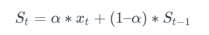
amongRepresents the smoothing value of the current time and the previous time, tableShow the actual value at the current time, α Represents the smoothing coefficient. The larger the coefficient, the greater the influence of the nearest neighbor's data.

Holt Exponential Smoothing, by introducing an additional coefficient, solves the problem that exponential smoothing cannot be applied to data with trend characteristics, but it still cannot solve the smoothing problem of data with seasonal changes.

Holt winters exponential smoothing, which solves the problem that Holt Exponential Smoothing cannot solve the problem of seasonal variation data by introducing a new coefficient again. In short, it is realized by introducing trend coefficient and seasonal coefficient on the basis of exponential smoothing with only one smoothing coefficient. This technology is widely used in time series prediction (such as future sales data prediction).

Python implements exponential smoothing

# Import air passenger data
air = pd.read_csv('data\\air.csv')
# Sets two smoothing factors
air['smooth_0.5']= air.Passengers.ewm(alpha =0.5).mean()
air['smooth_0.9']= air.Passengers.ewm(alpha =0.9).mean()
# Visual presentation
plt.plot(air.Date,air.Passengers,label='actual')
plt.plot(air.Date,air['smooth_0.5'],label='alpha=0.5')
plt.plot(air.Date,air['smooth_0.9'],label='alpha=0.9')
plt.xticks(rotation=45)
plt.legend()