Graph structure can be seen everywhere in the real world. Roads, social networks and molecular structures can be represented by graphs. Graph is one of the most important data structures we have.

There are many resources today that can teach us everything we need to apply machine learning to such data.
There have been many theories and materials about graph machine learning, especially graph neural networks, so this paper will avoid explaining these contents here. If you are not familiar with this aspect, it is recommended to take a look at CS224W first, which will be very helpful for you to get started.

This article uses pytorch geometry to implement the model we need, so the first step is to install

try:
    # Check if PyTorch Geometric is installed:
    import torch_geometric
except ImportError:
    # If PyTorch Geometric is not installed, install it.
    %pip install -q torch-scatter -f https://pytorch-geometric.com/whl/torch-1.7.0+cu101.html
    %pip install -q torch-sparse -f https://pytorch-geometric.com/whl/torch-1.7.0+cu101.html
    %pip install -q torch-geometric

After installation, import the package we need

from typing import Callable, List, Optional, Tuple

import matplotlib.pyplot as plt
import numpy as np
import torch
import torch.nn.functional as F
import torch_geometric.transforms as T
from torch import Tensor
from torch.optim import Optimizer
from torch_geometric.data import Data
from torch_geometric.datasets import Planetoid
from torch_geometric.nn import GCNConv
from torch_geometric.utils import accuracy
from typing_extensions import Literal, TypedDict

Cora dataset

The Cora dataset contains 2708 scientific publications, which are divided into one of seven categories. The referenced network consists of 5429 links. Each publication in the dataset is described by a word vector with a value of 0 / 1, which indicates whether the corresponding word in the dictionary exists. The dictionary contains 1433 unique words.

First, let's explore this dataset to see how it is generated:

dataset = Planetoid("/tmp/Cora", name="Cora")
num_nodes = dataset.data.num_nodes
# For num. edges see:
# - https://github.com/pyg-team/pytorch_geometric/issues/343
# - https://github.com/pyg-team/pytorch_geometric/issues/852
num_edges = dataset.data.num_edges // 2
train_len = dataset[0].train_mask.sum()
val_len = dataset[0].val_mask.sum()
test_len = dataset[0].test_mask.sum()
other_len = num_nodes - train_len - val_len - test_len
print(f"Dataset: {dataset.name}")
print(f"Num. nodes: {num_nodes} (train={train_len}, val={val_len}, test={test_len}, other={other_len})")
print(f"Num. edges: {num_edges}")
print(f"Num. node features: {dataset.num_node_features}")
print(f"Num. classes: {dataset.num_classes}")
print(f"Dataset len.: {dataset.len()}")

output

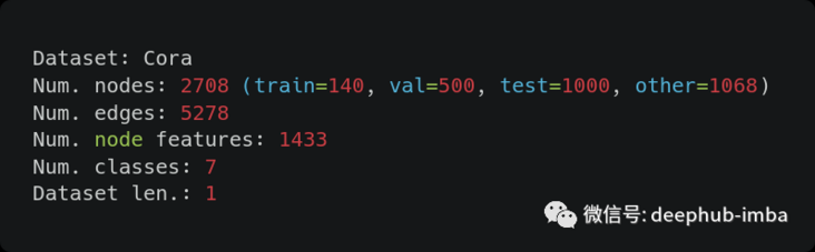
We can see some information:

• In order to get the correct number of edges, we must divide the data attribute "num_edges" by 2, because pytorch geometry "saves each link as an undirected edge in two directions".
• After doing so, the number is not right. Obviously, it is because "Cora dataset has duplicate edges", which requires us to clean the data
• Another strange fact is that after removing the nodes used for training, verification and testing, there are other nodes.
• Finally, we can see that the Cora dataset actually contains only one graph.

We use the initialization described in glorot & bengio (2010) to initialize the weights and normalize the input eigenvectors accordingly (rows). (kipf & welling ICLR 2017 arXiv: 1609.02907)

Glorot initialization is completed by pytorch geometry by default. The purpose of row normalization is to make the sum of features of each node 1, so we must explicitly process it:

dataset = Planetoid("/tmp/Cora", name="Cora")
print(f"Sum of row values without normalization: {dataset[0].x.sum(dim=-1)}")

dataset = Planetoid("/tmp/Cora", name="Cora", transform=T.NormalizeFeatures())
print(f"Sum of row values with normalization: {dataset[0].x.sum(dim=-1)}")

The output is as follows:

Figure convolution network GCN

Now that we have the data, it's time to define our graph convolution network (GCN)!

class GCN(torch.nn.Module):
    def __init__(
        self,
        num_node_features: int,
        num_classes: int,
        hidden_dim: int = 16,
        dropout_rate: float = 0.5,
    ) -> None:
        super().__init__()
        self.dropout1 = torch.nn.Dropout(dropout_rate)
        self.conv1 = GCNConv(num_node_features, hidden_dim)
        self.relu = torch.nn.ReLU(inplace=True)
        self.dropout2 = torch.nn.Dropout(dropout_rate)
        self.conv2 = GCNConv(hidden_dim, num_classes)

    def forward(self, x: Tensor, edge_index: Tensor) -> torch.Tensor:
        x = self.dropout1(x)
        x = self.conv1(x, edge_index)
        x = self.relu(x)
        x = self.dropout2(x)
        x = self.conv2(x, edge_index)
        return x
print("Graph Convolutional Network (GCN):")
GCN(dataset.num_node_features, dataset.num_classes)

If you look at the implementation in the pytorch geometry document, or even Thomas Kipf's implementation in the framework, you will find some inconsistencies (for example, there are two dropout layers). In fact, this is because neither of them is completely the same as the original implementation in TensorFlow, so we don't consider the original implementation here and only use the model provided by pytorch geometry.

Training and evaluation

Before training, we prepare the training and evaluation steps:

LossFn = Callable[[Tensor, Tensor], Tensor]
Stage = Literal["train", "val", "test"]

def train_step(
    model: torch.nn.Module, data: Data, optimizer: torch.optim.Optimizer, loss_fn: LossFn
) -> Tuple[float, float]:
    model.train()
    optimizer.zero_grad()
    mask = data.train_mask
    logits = model(data.x, data.edge_index)[mask]
    preds = logits.argmax(dim=1)
    y = data.y[mask]
    loss = loss_fn(logits, y)
    # + L2 regularization to the first layer only
    # for name, params in model.state_dict().items():
    #     if name.startswith("conv1"):
    #         loss += 5e-4 * params.square().sum() / 2.0

    acc = accuracy(preds, y)
    loss.backward()
    optimizer.step()
    return loss.item(), acc

@torch.no_grad()
def eval_step(model: torch.nn.Module, data: Data, loss_fn: LossFn, stage: Stage) -> Tuple[float, float]:
    model.eval()
    mask = getattr(data, f"{stage}_mask")
    logits = model(data.x, data.edge_index)[mask]
    preds = logits.argmax(dim=1)
    y = data.y[mask]
    loss = loss_fn(logits, y)
    # + L2 regularization to the first layer only
    # for name, params in model.state_dict().items():
    #     if name.startswith("conv1"):
    #         loss += 5e-4 * params.square().sum() / 2.0

    acc = accuracy(preds, y)
    return loss.item(), acc

The model takes the whole graph as input, and the mask of output and target depends on training, verification or test.

Or from kipf & welling (ICLR 2017): we use Adam (Kingma & Ba, 2015) to train all models for up to 200 rounds, with a learning rate of 0.01, and use the early stop mechanism with a window size of 10, that is, if the loss of 10 consecutive epoch s is not reduced, we will stop the training.

Some of the code here has been commented out and not really used because it attempts to apply L2 regularization only to the first layer in the original implementation. In general, PyTorch cannot easily replicate all the work in TensorFlow 100%, so in this example, the best tested is the Adam optimizer using weight attenuation.

class HistoryDict(TypedDict):
    loss: List[float]
    acc: List[float]
    val_loss: List[float]
    val_acc: List[float]

def train(
    model: torch.nn.Module,
    data: Data,
    optimizer: torch.optim.Optimizer,
    loss_fn: LossFn = torch.nn.CrossEntropyLoss(),
    max_epochs: int = 200,
    early_stopping: int = 10,
    print_interval: int = 20,
    verbose: bool = True,
) -> HistoryDict:
    history = {"loss": [], "val_loss": [], "acc": [], "val_acc": []}
    for epoch in range(max_epochs):
        loss, acc = train_step(model, data, optimizer, loss_fn)
        val_loss, val_acc = eval_step(model, data, loss_fn, "val")
        history["loss"].append(loss)
        history["acc"].append(acc)
        history["val_loss"].append(val_loss)
        history["val_acc"].append(val_acc)
        # The official implementation in TensorFlow is a little different from what is described in the paper...
        if epoch > early_stopping and val_loss > np.mean(history["val_loss"][-(early_stopping + 1) : -1]):
            if verbose:
                print("\nEarly stopping...")

            break

        if verbose and epoch % print_interval == 0:
            print(f"\nEpoch: {epoch}\n----------")
            print(f"Train loss: {loss:.4f} | Train acc: {acc:.4f}")
            print(f"  Val loss: {val_loss:.4f} |   Val acc: {val_acc:.4f}")

    test_loss, test_acc = eval_step(model, data, loss_fn, "test")
    if verbose:
        print(f"\nEpoch: {epoch}\n----------")
        print(f"Train loss: {loss:.4f} | Train acc: {acc:.4f}")
        print(f"  Val loss: {val_loss:.4f} |   Val acc: {val_acc:.4f}")
        print(f" Test loss: {test_loss:.4f} |  Test acc: {test_acc:.4f}")

    return history
def plot_history(history: HistoryDict, title: str, font_size: Optional[int] = 14) -> None:
    plt.suptitle(title, fontsize=font_size)
    ax1 = plt.subplot(121)
    ax1.set_title("Loss")
    ax1.plot(history["loss"], label="train")
    ax1.plot(history["val_loss"], label="val")
    plt.xlabel("Epoch")
    ax1.legend()

    ax2 = plt.subplot(122)
    ax2.set_title("Accuracy")
    ax2.plot(history["acc"], label="train")
    ax2.plot(history["val_acc"], label="val")
    plt.xlabel("Epoch")
    ax2.legend()

It should be noted that the early stop logic described in the paper is slightly different from the official implementation: it is not that the verification loss does not reduce the average value of the last ten values, but stops when it is greater.

Now let's start training

SEED = 42
MAX_EPOCHS = 200
LEARNING_RATE = 0.01
WEIGHT_DECAY = 5e-4
EARLY_STOPPING = 10

torch.manual_seed(SEED)
device = torch.device("cuda" if torch.cuda.is_available() else "cpu")

model = GCN(dataset.num_node_features, dataset.num_classes).to(device)
data = dataset[0].to(device)
optimizer = torch.optim.Adam(model.parameters(), lr=LEARNING_RATE, weight_decay=WEIGHT_DECAY)
history = train(model, data, optimizer, max_epochs=MAX_EPOCHS, early_stopping=EARLY_STOPPING)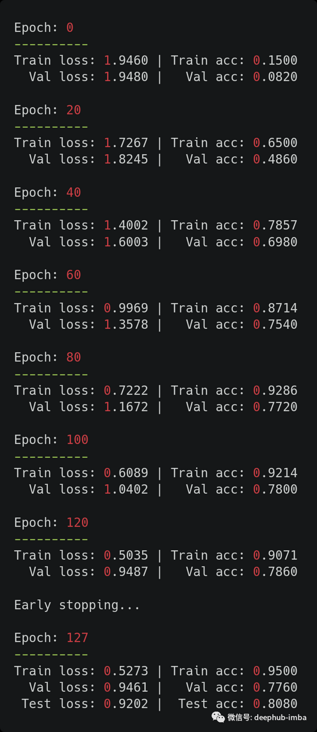

The results are also good. We obtained the test accuracy consistent with that reported in the original paper (81.5% in the paper). Because this is a small data set, these results are very sensitive to the selected random seeds. One solution to alleviate this problem is to average 100 (or more) runs like the author.

Finally, let's look at the loss and accuracy curve.

plt.figure(figsize=(12, 4))
plot_history(history, "GCN")

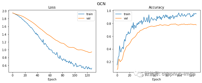
Although the verification loss continued to decline for a longer time, the verification accuracy has actually stabilized since round 20.

quote

Original paper:

Semi-Supervised Classification with Graph Convolutional Networks : https://arxiv.org/abs/1609.02907

PyG (PyTorch Geometric) document: https://pytorch-geometric.rea...

Author: Mario Namtao Shianti Larcher