Through the previous practice of in-depth learning, whether it is the CNN network built by ourselves or the official network model called through migration learning, it has its advantages and disadvantages. This experiment calls various common CNN network models to understand their characteristics and compare the accuracy of classification for the same data set.
The CNN models called this time include: vgg16 vgg19 RESNET intensity model

1. Import library

import tensorflow as tf
import numpy as np
import matplotlib.pyplot as plt
import os,PIL,pathlib
from tensorflow import keras
from tensorflow.keras import layers,models,Sequential,Input

2. Load data

The operation is similar to that before. The data is divided into training set and test set according to the ratio of 8:2

data_dir = "E:/tmp/.keras/datasets/Pokemon_photos"
data_dir = pathlib.Path(data_dir)

img_count = len(list(data_dir.glob('*/*.png')))#219 photos in total
# print(img_count)

height = 224
width = 224
epochs = 20
batch_size = 8
train_data_gen = tf.keras.preprocessing.image.ImageDataGenerator(
    rescale=1./255,
    rotation_range=45,
    shear_range=0.2,
    zoom_range=0.2,
    validation_split=0.2,
    horizontal_flip=True
)
train_ds = train_data_gen.flow_from_directory(
    directory=data_dir,
    target_size=(height,width),
    batch_size=batch_size,
    shuffle=True,
    class_mode='categorical',
    subset='training'
)
test_ds = train_data_gen.flow_from_directory(
    directory=data_dir,
    target_size=(height,width),
    batch_size=batch_size,
    shuffle=True,
    class_mode='categorical',
    subset='validation'
)

3. Build your own CNN network

Three layer convolution pool layer + Flatten + three-layer full connection layer

#CNN
model = tf.keras.Sequential([
    tf.keras.layers.Conv2D(16,3,padding="same",activation="relu",input_shape=(height,width,3)),
    tf.keras.layers.MaxPooling2D(),
    tf.keras.layers.Conv2D(32,3,padding="same",activation="relu"),
    tf.keras.layers.MaxPooling2D(),
    tf.keras.layers.Conv2D(64,3,padding="same",activation="relu"),
    tf.keras.layers.AveragePooling2D(),
    tf.keras.layers.Flatten(),
    tf.keras.layers.Dense(1024,activation="relu"),
    tf.keras.layers.Dense(512,activation="relu"),
    tf.keras.layers.Dense(10,activation="softmax")
])

The final model accuracy rate is about 80%. Through the experimental results, it can be found that increasing the number of epochs, the final model accuracy rate is not improved, but in shock, and the highest model accuracy rate is when epochs is 20.

4. Official model

VGG16 model
VGG16 and VGG19 are the two most classic models in VGG series, and the latter has a deeper level. VGG series models have the following characteristics:
① Small convolution kernel: compared with AlexNet, all convolution kernels are replaced with 3x3, and 1x1 is rarely used. 3x3 is the smallest size that can capture eight neighborhood information of pixels.
② Small pool layer: compared with AlexNet, 3x3 pool cores are replaced by 2x2 pool cores.
③ The number of layers is deeper: VGG16, for example, 3 → 64 → 126 → 256 → 512. The convolution core focuses on expanding the number of channels. The features of the three channels are extracted and diffused to 512 channels through the convolution layer.
④ The number of layers is deeper: VGG16, for example, 3 → 64 → 126 → 256 → 512. The convolution core focuses on expanding the number of channels. The features of the three channels are extracted and diffused to 512 channels through the convolution layer.
⑤ Full connection to 1 × 1 convolution: input of any width or height can be received in the test stage.
This is a change compared with the previous model of VGG model, so why do you make such a change?

3x3 convolution kernel
The limited receptive field of two 3x3 stacked volumes is 5x5; The receptive field of three 3x3 stacked convolution base layers is 7x7, so the stacking of small-size convolution layers can replace large-size convolution layers, and the receptive field size remains unchanged. Multiple small convolutions can extract larger and deeper convolution features and reduce the number of model parameters.

2x2 pool core
The maximum pool core of AlexNet is 3 × 3. The stride is 2. VGGNet maximum pool core is 2 × 2. The stride is 2 22. The small pool core brings more detailed information capture.

1x1 convolution kernel
In the test phase, the input with any width or height can be received to eliminate the input limitation.

Call the official VGG16 model, and several common parameters are explained as follows:

VGG All parameters contained in the model are similar in other official models.
tf.keras.applications.vgg16.VGG16(
    include_top=True, weights='imagenet', input_tensor=None,
    input_shape=None, pooling=None, classes=1000,
    classifier_activation='softmax'
)

include_top: Whether the three full connection layers at the top of the network are included.
weights: The weight file is not loaded by default,"imagenet"Load the official weight file, or enter your own weight file path.
classes: Number of categories that classify images.

conv_base = tf.keras.applications.VGG16(weights = 'imagenet',include_top = False)
conv_base.trainable =False#Untrained
#Model building
model = tf.keras.Sequential()
model.add(conv_base)
model.add(tf.keras.layers.GlobalAveragePooling2D())
model.add(tf.keras.layers.Dense(1024,activation='relu'))
model.add(tf.keras.layers.Dense(10,activation='softmax'))

Configuration and of optimizer Previous blogs The settings of are the same and will not be repeated here.

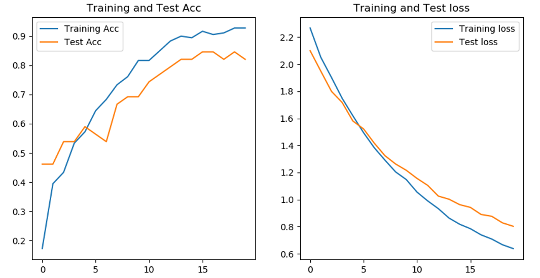
Compared with the CNN network built by ourselves, the accuracy of VGG16 model does not vibrate so frequently, and the final accuracy of the model is 80%. However, under the condition of epochs=20, the training effect should be better under the same condition of epochs.

Call the official VGG19 model

conv_base = tf.keras.applications.VGG19(weights = 'imagenet',include_top = False)
conv_base.trainable =False#Untrained
#Model building
model = tf.keras.Sequential()
model.add(conv_base)
model.add(tf.keras.layers.GlobalAveragePooling2D())
model.add(tf.keras.layers.Dense(1024,activation='relu'))
model.add(tf.keras.layers.Dense(10,activation='softmax'))

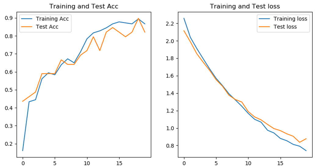
Compared with VGG16 model, VGG19 model fully reflects the benefits of deepening network depth for model accuracy. The accuracy of the model is more than 80%, and the highest is 90%.

ResNet50 model

On the premise that the deep network can converge, with the increase of network depth, the accuracy begins to saturate or even decline, which is called the network degradation problem. To some extent, deepening the network model can increase the accuracy of the model, but if the network depth is too deep, the accuracy will decline. These degradation are not caused by over fitting. Under extreme conditions, If all the added layers are the direct copy of the previous layer (i.e. y=x), the training error of the deep network should be equal to that of the shallow network. Therefore, the root cause of network degradation is the optimization problem. In order to solve the optimization problem, a residual network is proposed. The residual network can be understood as adding some quick connections to the forward network (shortcut connections). These connections will skip some layers and directly transfer the original data to subsequent layers. The new quick connections will not increase the parameters and complexity of the model. The whole model can still be trained by end-to-end methods (such as SGD), which is not difficult to implement.

conv_base = tf.keras.applications.ResNet50(weights = 'imagenet',include_top = False)
conv_base.trainable =False
#Model building
model = tf.keras.Sequential()
model.add(conv_base)
model.add(tf.keras.layers.GlobalAveragePooling2D())
model.add(tf.keras.layers.Dense(1024,activation='relu'))
model.add(tf.keras.layers.Dense(10,activation='softmax'))

This result is very confusing. The accuracy of the training set has been as high as 100%, but the accuracy of the test set is almost 0. It shouldn't be the problem of the network itself. Bloggers don't quite understand the setting of some parameters. I hope the big guys passing by can give some advice. In a previous blog Bird identification At that time, it was thought to be over fitting, but now it doesn't seem to be over fitting.

Densenet model

This model is a network model proposed in recent years. It is not commonly used, but its advantages are prominent.
1. Reduced vanishing gradient
2. Enhance the transfer of feature s.
3. More efficient use of feature s.
4. The number of parameters is reduced to some extent.

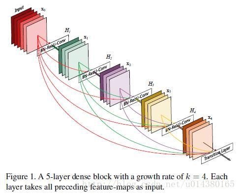
Densenet model directly connects all layers on the premise of ensuring the maximum information transmission between middle layers of the network! In the traditional convolutional neural network, if you have l layers, there will be l connections, but in densenet, there will be L(L+1)/2 connections. In short, the input of each layer comes from the output of all previous layers. as Figure below As shown in:

conv_base = tf.keras.applications.densenet.DenseNet121(weights = 'imagenet',include_top = False)
conv_base.trainable =False
#Model building
model = tf.keras.Sequential()
model.add(conv_base)
model.add(tf.keras.layers.GlobalAveragePooling2D())
model.add(tf.keras.layers.Dense(1024,activation='relu'))
model.add(tf.keras.layers.Dense(10,activation='softmax'))

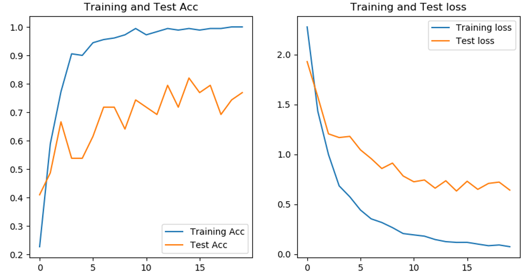
The accuracy of the network in the training set has reached 98%, but the accuracy of the test set is between 70% - 80%, which is not as high as that of the VGG model.

Summary:
This paper only compares the accuracy of using different network models for the same data set, and does not say that a certain network model must be good. Any kind of network model has its outstanding advantages and disadvantages. In the recognition of magic baby, VGG19 network has the highest accuracy, and there is no vibration or over fitting.