 What do I know What do I know |  My WeChat official account My WeChat official account |  My CSDN My CSDN |  Download this article source code + data Download this article source code + data |  Need help Need help |
In this tutorial, you will learn how to use migration learning to classify images of cats and dogs through a pre training network.
The pre training model is a saved network previously trained based on large data sets (usually large image classification tasks).
Transfer learning is usually applied to too few data sets to effectively complete the training of the model. Therefore, we seek to train and fine tune on the basis of the pre training model to solve this problem. Of course, even if the data set is not so small, we can speed up the training of the model by pre training the model.
In this paper, we do not need to (RE) train the whole model. The basic convolutional network already contains the features commonly used for image classification. However, the final classification part of the pre training model is specific to the original classification task, and then specific to the class set used by the training model.
- Fine tuning: unfreeze some top layers of the frozen model library, and jointly train the newly added classifier layer and the last layers of the basic model. In this way, we can "fine tune" the high-order feature representation in the base model to make it more relevant to specific tasks (migrated tasks).
Will follow the general workflow of deep learning.
- Check and understand data
- Build the input pipeline, in this case using Keras ImageDataGenerator
- Constitutive model
- Load the basic model of pre training (and pre training weight)
- Stack classification layers on top
- Training model
- Evaluation model
from tensorflow.keras.preprocessing import image_dataset_from_directory
import matplotlib.pyplot as plt
import numpy as np
import os

#Set the amount of GPU video memory and use it on demand
import tensorflow as tf
gpus = tf.config.list_physical_devices("GPU")

if gpus:
    tf.config.experimental.set_memory_growth(gpus[0], True)
    tf.config.set_visible_devices([gpus[0]],"GPU")

#Ignore warning messages
import warnings
warnings.filterwarnings("ignore")
Data preprocessing
Data download
In this tutorial, you will use a dataset containing thousands of cat and dog images. Download and unzip the zip file containing the image, and then use tf.keras.preprocessing.image_ dataset_ from_ The directory utility function creates a tf.data.Dataset for training and verification.
_URL = 'https://storage.googleapis.com/mledu-datasets/cats_and_dogs_filtered.zip'
path_to_zip = tf.keras.utils.get_file('cats_and_dogs.zip', origin=_URL, extract=True)
PATH = os.path.join(os.path.dirname(path_to_zip), 'cats_and_dogs_filtered')

train_dir = os.path.join(PATH, 'train')
validation_dir = os.path.join(PATH, 'validation')

BATCH_SIZE = 32
IMG_SIZE = (160, 160)

train_dataset = image_dataset_from_directory(train_dir,
                                             shuffle=True,
                                             batch_size=BATCH_SIZE,
                                             image_size=IMG_SIZE)
Downloading data from https://storage.googleapis.com/mledu-datasets/cats_and_dogs_filtered.zip
68608000/68606236 [==============================] - 14s 0us/step
Found 2000 files belonging to 2 classes.
validation_dataset = image_dataset_from_directory(validation_dir,
                                                  shuffle=True,
                                                  batch_size=BATCH_SIZE,
                                                  image_size=IMG_SIZE)
Found 1000 files belonging to 2 classes.
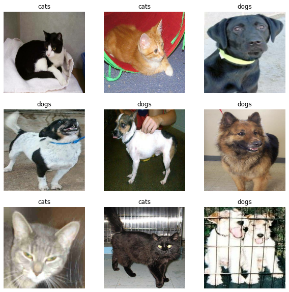
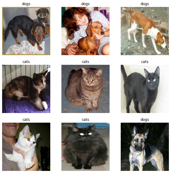
Display the first nine images and labels in the training set:
class_names = train_dataset.class_names

plt.figure(figsize=(10, 10))
for images, labels in train_dataset.take(1):
    for i in range(9):
        ax = plt.subplot(3, 3, i + 1)
        plt.imshow(images[i].numpy().astype("uint8"))
        plt.title(class_names[labels[i]])
        plt.axis("off")
Since the original dataset does not contain a test set, you need to create one. To do this, use tf.data.experimental.cardinality to determine how many batches of data are in the validation set, and then move 20% of them to the test set.
val_batches        = tf.data.experimental.cardinality(validation_dataset)
test_dataset       = validation_dataset.take(val_batches // 5)
validation_dataset = validation_dataset.skip(val_batches // 5)
print('Number of validation batches: %d' % tf.data.experimental.cardinality(validation_dataset))
print('Number of test batches: %d' % tf.data.experimental.cardinality(test_dataset))
Number of validation batches: 26
Number of test batches: 6
Configure datasets to improve performance
Use buffer pre extraction to load images from disk to avoid I/O blocking.
AUTOTUNE = tf.data.AUTOTUNE

train_dataset      = train_dataset.prefetch(buffer_size=AUTOTUNE)
validation_dataset = validation_dataset.prefetch(buffer_size=AUTOTUNE)
test_dataset       = test_dataset.prefetch(buffer_size=AUTOTUNE)
Using data expansion
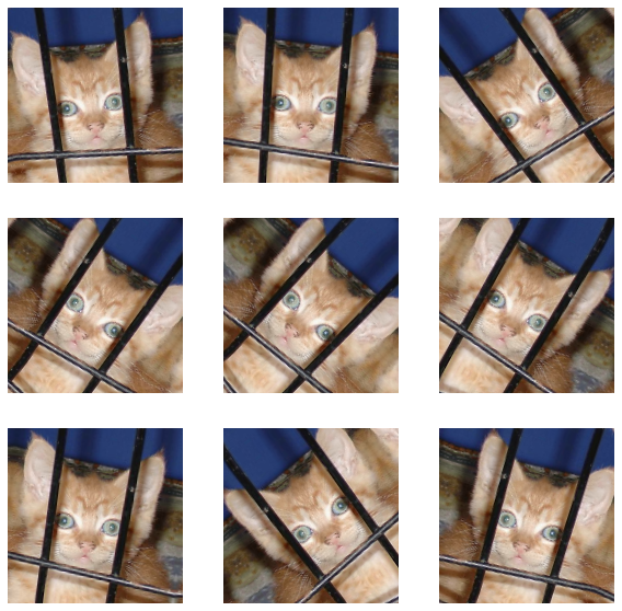
When you don't have a large image data set, it's best to apply random but realistic transformation to the training image (such as rotation or horizontal flip) to artificially introduce sample diversity. This helps expose the model to different aspects of the training data and reduce Over fitting . You can be here course Learn more about data expansion in.
data_augmentation = tf.keras.Sequential([
  tf.keras.layers.experimental.preprocessing.RandomFlip('horizontal'),
  tf.keras.layers.experimental.preprocessing.RandomRotation(0.2),
])
Note: when you call model.fit, these layers are only valid during training. When models are used in inference mode in model.evaluate or model.fit, they are disabled.
We apply these layers repeatedly to the same image, and then look at the results.
for image, _ in train_dataset.take(1):
    plt.figure(figsize=(10, 10))
    first_image = image[0]
    for i in range(9):
        ax = plt.subplot(3, 3, i + 1)
        augmented_image = data_augmentation(tf.expand_dims(first_image, 0))
        plt.imshow(augmented_image[0] / 255)
        plt.axis('off')
Rescale pixel values
Later, you will download tf.keras.applications.MobileNetV2 as the base model. This model expects the pixel value to be in the range of [- 1,1], but at this time, the pixel value in the image is in the range of [0,255]. To rescale these pixel values, use the preprocessing method that comes with the model.
"""
about tf.keras.applications.mobilenet_v2.preprocess_input

The official original text of the return value: The inputs pixel values are scaled between -1 and 1, sample-wise.
Function function: shrink pixel value to[-1,1]between
"""
preprocess_input = tf.keras.applications.mobilenet_v2.preprocess_input
Note: in addition, you can also use Rescaling The layer rescaled the pixel value from [0255] to [- 1, 1].
rescale = tf.keras.layers.experimental.preprocessing.Rescaling(1./127.5, offset= -1)

"""
If you want to shrink[0,1]It can be written like this
rescale = tf.keras.layers.experimental.preprocessing.Rescaling(scale=1./255)
"""
Creating a basic model from a pre trained convolutional network
You will create the base model based on the MobileNet V2 model developed by Google. This model has been pre trained based on ImageNet dataset, which is a large dataset containing 1.4 million images and 1000 classes. ImageNet is a research training dataset with a variety of categories, such as jackfruit and syringe. This knowledge base will help us classify cats and dogs in a specific dataset.
First, you need to choose which layer of MobileNet V2 is used for feature extraction. The final classification layer (at the "top" because most machine learning model diagrams are bottom-up) is not very useful. Instead, you will rely on the last layer before the flattening operation as usual. This layer is called the "bottleneck layer". Compared with the last layer / top layer, the characteristics of the bottleneck layer retain more generality.
First, instantiate a MobileNet V2 model with pre loaded weights based on ImageNet training. By specifying include_ The top = false parameter can load networks that do not include the top classification layer, which is ideal for feature extraction.
# Create a base model using official weights
IMG_SHAPE = IMG_SIZE + (3,)
base_model = tf.keras.applications.MobileNetV2(input_shape=IMG_SHAPE,
                                               include_top=False,
                                               weights='imagenet')
This feature extraction program converts each 160x160x3 image into a 5x5x1280 feature block. Let's see what it does with a batch of sample images:
image_batch, label_batch = next(iter(train_dataset))
feature_batch = base_model(image_batch)
print(feature_batch.shape)
(32, 5, 5, 1280)
feature extraction
In this step, you will freeze the convolution base created in the previous step and use it as a feature extractor. In addition, you can add classifiers at the top and train top-level classifiers.
Frozen convolution basis
It is very important to freeze the convolution basis before compiling and training the model. Freezing (by setting layer.trainable = False) avoids updating weights in a given layer during training. MobileNet V2 has many layers, so setting the trainable flag of the entire model to False freezes all these layers.
base_model.trainable = False
Important notes on the BatchNormalization layer
Many models contain tf.keras.layers.BatchNormalization layers. This layer is a special case and precautions should be taken in the context of fine tuning, as shown later in this tutorial.
When layer.trainable = False is set, the BatchNormalization layer runs in inference mode and its mean and variance statistics are not updated.
When thawing a model containing a BatchNormalization layer for fine tuning, keep the BatchNormalization layer in inference mode by passing training = False when calling base model. Otherwise, updates applied to untrained weights will destroy what the model has learned.
# Print base model structure
base_model.summary()
Model: "mobilenetv2_1.00_160"
__________________________________________________________________________________________________
Layer (type)                    Output Shape         Param #     Connected to
==================================================================================================
input_1 (InputLayer)            [(None, 160, 160, 3) 0
__________________________________________________________________________________________________
Conv1 (Conv2D)                  (None, 80, 80, 32)   864         input_1[0][0]
__________________________________________________________________________________________________
bn_Conv1 (BatchNormalization)   (None, 80, 80, 32)   128         Conv1[0][0]
......
__________________________________________________________________________________________________
Conv_1_bn (BatchNormalization)  (None, 5, 5, 1280)   5120        Conv_1[0][0]
__________________________________________________________________________________________________
out_relu (ReLU)                 (None, 5, 5, 1280)   0           Conv_1_bn[0][0]
==================================================================================================
Total params: 2,257,984
Trainable params: 0
Non-trainable params: 2,257,984
__________________________________________________________________________________________________
Add category header
To generate a prediction from a feature block, use the tf.keras.layers.GlobalAveragePooling2D layer to average in 5x5 spatial positions to convert the feature into a vector (containing 1280 elements) per image.
global_average_layer = tf.keras.layers.GlobalAveragePooling2D()
feature_batch_average = global_average_layer(feature_batch)
print(feature_batch_average.shape)
(32, 1280)
The tf.keras.layers.Dense layer is applied to convert these features into a prediction for each image. You do not need to activate the function here because this prediction will be treated as logit or the original prediction value. Positive numbers predict category 1 and negative numbers predict category 0.
prediction_layer = tf.keras.layers.Dense(1)
prediction_batch = prediction_layer(feature_batch_average)
print(prediction_batch.shape)
(32, 1)
Expand, rescale, and base the data by using the Keras functional API_ Model and feature extractor layer are linked together to build the model. As mentioned earlier, since our model contains a BatchNormalization layer, please use training = False.
inputs = tf.keras.Input(shape=(160, 160, 3))
x = data_augmentation(inputs)
x = preprocess_input(x)
x = base_model(x, training=False)
x = global_average_layer(x)
x = tf.keras.layers.Dropout(0.2)(x)
outputs = prediction_layer(x)

model = tf.keras.Model(inputs, outputs)
Compilation model
Before training the model, you need to compile the model. Since there are two classes and the model provides linear output, compare the binary cross entropy loss with from_logits=True.
base_learning_rate = 0.0001
model.compile(optimizer=tf.keras.optimizers.Adam(lr=base_learning_rate),
              loss=tf.keras.losses.BinaryCrossentropy(from_logits=True),
              metrics=['accuracy'])
model.summary()
Model: "model"
_________________________________________________________________
Layer (type)                 Output Shape              Param #
=================================================================
input_2 (InputLayer)         [(None, 160, 160, 3)]     0
_________________________________________________________________
sequential (Sequential)      (None, 160, 160, 3)       0
_________________________________________________________________
tf.math.truediv (TFOpLambda) (None, 160, 160, 3)       0
_________________________________________________________________
tf.math.subtract (TFOpLambda (None, 160, 160, 3)       0
_________________________________________________________________
mobilenetv2_1.00_160 (Functi (None, 5, 5, 1280)        2257984
_________________________________________________________________
global_average_pooling2d (Gl (None, 1280)              0
_________________________________________________________________
dropout (Dropout)            (None, 1280)              0
_________________________________________________________________
dense (Dense)                (None, 1)                 1281
=================================================================
Total params: 2,259,265
Trainable params: 1,281
Non-trainable params: 2,257,984
_________________________________________________________________
2.5 million parameters in MobileNet are frozen, but there are 1200 trainable parameters in the dense layer. They are divided into two tf.Variable objects, weight and deviation.
len(model.trainable_variables)
2
Training model
After 10 cycles of training, you should see an accuracy of about 94% on the validation set.
initial_epochs = 10

loss0, accuracy0 = model.evaluate(validation_dataset)
26/26 [==============================] - 2s 25ms/step - loss: 0.8702 - accuracy: 0.4022
print("initial loss: {:.2f}".format(loss0))
print("initial accuracy: {:.2f}".format(accuracy0))
initial loss: 0.87
initial accuracy: 0.40
history = model.fit(train_dataset,
                    epochs=initial_epochs,
                    validation_data=validation_dataset)
Epoch 1/10
63/63 [==============================] - 4s 36ms/step - loss: 0.7913 - accuracy: 0.5070 - val_loss: 0.6019 - val_accuracy: 0.5928
Epoch 2/10
63/63 [==============================] - 2s 32ms/step - loss: 0.5866 - accuracy: 0.6730 - val_loss: 0.4355 - val_accuracy: 0.7574
Epoch 3/10
63/63 [==============================] - 2s 32ms/step - loss: 0.4451 - accuracy: 0.7695 - val_loss: 0.3383 - val_accuracy: 0.8243
Epoch 4/10
63/63 [==============================] - 2s 33ms/step - loss: 0.3875 - accuracy: 0.8225 - val_loss: 0.2799 - val_accuracy: 0.8639
Epoch 5/10
63/63 [==============================] - 2s 33ms/step - loss: 0.3350 - accuracy: 0.8345 - val_loss: 0.2273 - val_accuracy: 0.9097
Epoch 6/10
63/63 [==============================] - 2s 35ms/step - loss: 0.3062 - accuracy: 0.8640 - val_loss: 0.2028 - val_accuracy: 0.9097
Epoch 7/10
63/63 [==============================] - 2s 32ms/step - loss: 0.2765 - accuracy: 0.8840 - val_loss: 0.1758 - val_accuracy: 0.9319
Epoch 8/10
63/63 [==============================] - 2s 32ms/step - loss: 0.2538 - accuracy: 0.8925 - val_loss: 0.1613 - val_accuracy: 0.9418
Epoch 9/10
63/63 [==============================] - 2s 32ms/step - loss: 0.2478 - accuracy: 0.8845 - val_loss: 0.1472 - val_accuracy: 0.9455
Epoch 10/10
63/63 [==============================] - 2s 32ms/step - loss: 0.2301 - accuracy: 0.9015 - val_loss: 0.1351 - val_accuracy: 0.9493
learning curve
Let's look at the learning curve of training and verifying accuracy / loss when using MobileNet V2 basic model as a fixed feature extraction program.
acc = history.history['accuracy']
val_acc = history.history['val_accuracy']

loss = history.history['loss']
val_loss = history.history['val_loss']

plt.figure(figsize=(8, 8))
plt.subplot(2, 1, 1)
plt.plot(acc, label='Training Accuracy')
plt.plot(val_acc, label='Validation Accuracy')
plt.legend(loc='lower right')
plt.ylabel('Accuracy')
plt.ylim([min(plt.ylim()),1])
plt.title('Training and Validation Accuracy')

plt.subplot(2, 1, 2)
plt.plot(loss, label='Training Loss')
plt.plot(val_loss, label='Validation Loss')
plt.legend(loc='upper right')
plt.ylabel('Cross Entropy')
plt.ylim([0,1.0])
plt.title('Training and Validation Loss')
plt.xlabel('epoch')
plt.show()
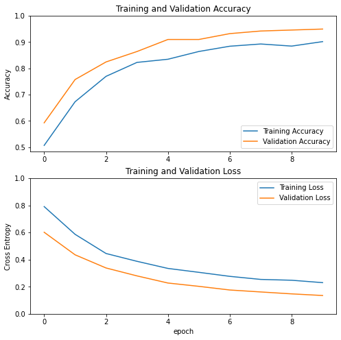
Note: if you want to know why the verification index is obviously better than the training index, the main reason is that the tf.keras.layers.BatchNormalization and tf.keras.layers.Dropout will affect the accuracy during training. They are closed when calculating the verification loss.
To a lesser extent, this is also because the training index reports the average value of a certain cycle, while the verification index is evaluated after the cycle, so the verification index will see the model with slightly longer training time.
Fine tuning
In the feature extraction experiment, you only trained some layers at the top of the MobileNet V2 basic model. The weight of the pre training network is not updated during the training process.
One way to further improve performance is to train (or "fine tune") the weights at the top level of the pre training model, as well as the classifiers you add. The training process adjusts the mandatory weight from the general feature mapping to the features specifically associated with the data set.
Note: you can only try to do this after you train the top-level classifier with a pre training model that is set as untrainable. If you add a randomly initialized classifier at the top of the pre training model and try to train all layers together, the gradient update will be too large (due to the random weight of the classifier), which will cause your pre training model to forget what it has learned.
In addition, you should try to fine tune a small number of top layers rather than the entire MobileNet model. In most convolution networks, the higher the layer, the higher its specialization. The first few layers learn very simple and general features, which can be generalized to almost all types of images. As you move up, these characteristics become more and more specific to the dataset used by the training model. The goal of fine tuning is to adapt these special features to the new data set, rather than covering general learning.
Thaw the top layer of the model
What you need to do is unfreeze the base_model and set the bottom layer as untrainable. You should then recompile the model (what is necessary for these changes to take effect) and resume training.
base_model.trainable = True
# Print the total number of layer s in the base model
print("Number of layers in the base model: ", len(base_model.layers))

# Fine tune fine_ tune_ layer after at
fine_tune_at = 100

# Freeze fine_ tune_ All layer s before at
for layer in base_model.layers[:fine_tune_at]:
    layer.trainable =  False
Number of layers in the base model: 154
Compilation model
When you are training a much larger model and want to readjust the pre training weights, be sure to use a lower learning rate at this stage. Otherwise, your model may over fit quickly.
model.compile(loss=tf.keras.losses.BinaryCrossentropy(from_logits=True),
              optimizer = tf.keras.optimizers.RMSprop(lr=base_learning_rate/10),
              metrics=['accuracy'])
model.summary()
Model: "model"
_________________________________________________________________
Layer (type)                 Output Shape              Param #
=================================================================
input_2 (InputLayer)         [(None, 160, 160, 3)]     0
_________________________________________________________________
sequential (Sequential)      (None, 160, 160, 3)       0
_________________________________________________________________
tf.math.truediv (TFOpLambda) (None, 160, 160, 3)       0
_________________________________________________________________
tf.math.subtract (TFOpLambda (None, 160, 160, 3)       0
_________________________________________________________________
mobilenetv2_1.00_160 (Functi (None, 5, 5, 1280)        2257984
_________________________________________________________________
global_average_pooling2d (Gl (None, 1280)              0
_________________________________________________________________
dropout (Dropout)            (None, 1280)              0
_________________________________________________________________
dense (Dense)                (None, 1)                 1281
=================================================================
Total params: 2,259,265
Trainable params: 1,862,721
Non-trainable params: 396,544
_________________________________________________________________
len(model.trainable_variables)
56
Continuous training model
If you have trained to convergence in advance, this step will improve your accuracy by several percentage points.
fine_tune_epochs = 10
total_epochs =  initial_epochs + fine_tune_epochs

history_fine = model.fit(train_dataset,
                         epochs=total_epochs,
                         initial_epoch=history.epoch[-1],
                         validation_data=validation_dataset)
Epoch 10/20
63/63 [==============================] - 8s 62ms/step - loss: 0.1459 - accuracy: 0.9345 - val_loss: 0.0524 - val_accuracy: 0.9814
Epoch 11/20
63/63 [==============================] - 3s 50ms/step - loss: 0.1244 - accuracy: 0.9495 - val_loss: 0.0416 - val_accuracy: 0.9864
Epoch 12/20
63/63 [==============================] - 3s 49ms/step - loss: 0.1027 - accuracy: 0.9570 - val_loss: 0.0463 - val_accuracy: 0.9777
Epoch 13/20
63/63 [==============================] - 3s 50ms/step - loss: 0.0884 - accuracy: 0.9605 - val_loss: 0.0461 - val_accuracy: 0.9814
Epoch 14/20
63/63 [==============================] - 3s 50ms/step - loss: 0.0939 - accuracy: 0.9585 - val_loss: 0.0434 - val_accuracy: 0.9814
Epoch 15/20
63/63 [==============================] - 3s 50ms/step - loss: 0.0898 - accuracy: 0.9650 - val_loss: 0.0492 - val_accuracy: 0.9790
Epoch 16/20
63/63 [==============================] - 3s 50ms/step - loss: 0.0796 - accuracy: 0.9650 - val_loss: 0.0353 - val_accuracy: 0.9889
Epoch 17/20
63/63 [==============================] - 3s 51ms/step - loss: 0.0834 - accuracy: 0.9670 - val_loss: 0.0425 - val_accuracy: 0.9864
Epoch 18/20
63/63 [==============================] - 3s 50ms/step - loss: 0.0786 - accuracy: 0.9685 - val_loss: 0.0384 - val_accuracy: 0.9839
Epoch 19/20
63/63 [==============================] - 3s 50ms/step - loss: 0.0580 - accuracy: 0.9765 - val_loss: 0.0454 - val_accuracy: 0.9851
Epoch 20/20
63/63 [==============================] - 3s 51ms/step - loss: 0.0700 - accuracy: 0.9735 - val_loss: 0.0326 - val_accuracy: 0.9901
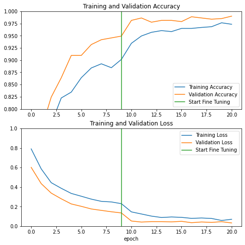
When fine tuning the last layers of the MobileNet V2 basic model and training classifiers on these layers, let's look at the learning curve of training and verifying accuracy / loss. The verification loss is much higher than the training loss, so there may be some over fitting.
When the new training set is relatively small and similar to the original MobileNet V2 data set, there may also be some over fitting.
After fine tuning, the accuracy of the model in the validation set is almost 98%.
acc += history_fine.history['accuracy']
val_acc += history_fine.history['val_accuracy']

loss += history_fine.history['loss']
val_loss += history_fine.history['val_loss']
plt.figure(figsize=(8, 8))
plt.subplot(2, 1, 1)
plt.plot(acc, label='Training Accuracy')
plt.plot(val_acc, label='Validation Accuracy')
plt.ylim([0.8, 1])
plt.plot([initial_epochs-1,initial_epochs-1],
          plt.ylim(), label='Start Fine Tuning')
plt.legend(loc='lower right')
plt.title('Training and Validation Accuracy')

plt.subplot(2, 1, 2)
plt.plot(loss, label='Training Loss')
plt.plot(val_loss, label='Validation Loss')
plt.ylim([0, 1.0])
plt.plot([initial_epochs-1,initial_epochs-1],
         plt.ylim(), label='Start Fine Tuning')
plt.legend(loc='upper right')
plt.title('Training and Validation Loss')
plt.xlabel('epoch')
plt.show()
Evaluation and prediction
Finally, you can use the test set to verify the performance of the model on new data.
loss, accuracy = model.evaluate(test_dataset)
print('Test accuracy :', accuracy)
6/6 [==============================] - 0s 20ms/step - loss: 0.0204 - accuracy: 0.9948
Test accuracy : 0.9947916865348816
Now, you can use this model to predict whether your pet is a cat or a dog.
#Retrieve a batch of images from the test set
image_batch, label_batch = test_dataset.as_numpy_iterator().next()
predictions = model.predict_on_batch(image_batch).flatten()

# Apply a sigmoid since our model returns logits
predictions = tf.nn.sigmoid(predictions)
predictions = tf.where(predictions < 0.5, 0, 1)

print('Predictions:\n', predictions.numpy())
print('Labels:\n', label_batch)

plt.figure(figsize=(10, 10))
for i in range(9):
    ax = plt.subplot(3, 3, i + 1)
    plt.imshow(image_batch[i].astype("uint8"))
    plt.title(class_names[predictions[i]])
    plt.axis("off")
Predictions:
 [1 1 1 0 0 0 0 0 1 0 1 0 1 0 0 0 0 1 0 1 1 1 0 1 0 0 1 0 1 0 0 0]
Labels:
 [1 1 1 0 0 0 0 0 1 0 1 0 1 0 0 0 0 1 0 1 1 1 0 1 0 0 1 0 1 0 0 0]
summary
-
Feature extraction using pre training model: when using small data sets, the common practice is to use the features learned by the model trained based on larger data sets in the same domain. To do this, you need to instantiate the pre training model and add a fully connected classifier at the top. The pre training model is in the "frozen state", and only the weight of the classifier is updated in the training process. In this case, the convolution basis extracts all the features associated with each image, and you have just trained a classifier to determine the image class according to the given extracted feature set.
-
Fine tuning the pre training model: in order to further improve the performance, it may be necessary to reuse the top level of the pre training model for new data sets through fine tuning. In this example, you adjusted the weights so that the model learns advanced features specific to the dataset. This technique is generally recommended when the training data set is large and very similar to the original data set used in the training pre training model.
Note: This article is taken from TensorFlow's official website and partially modified