This article is a supplement to the knowledge of pytorch before training Transformer. Thank blogger Mo fan for his video course on Python https://www.youtube.com/watch?v=lAaCeiqE6CE&feature=emb_title , whose home page is: Don't bother Python

It is recommended to directly watch the blogger's video tutorial to complete the knowledge supplement of pytorch. You can also browse my text records.

preface

Following the previous article, this is the last article of pytoch knowledge supplement. These parts are required for training Transformer and hardware design later, covering:

• How to build a network model
• Method of saving and extracting network
• Batch data training
• Batch normalization

1, Method of building network model

import torch
from torch.autograd import Variable
import torch.nn.functional as F
import matplotlib.pyplot as plt

#Building data sets
n_data = torch.ones(100,2)
x0 = torch.normal(2*n_data,0.6)
y0 = torch.zeros(100)
x1 = torch.normal(-2*n_data,0.6)
y1 = torch.ones(100)
x = torch.cat((x0,x1),0).type(torch.FloatTensor)#32bit float
y = torch.cat((y0,y1),).type(torch.LongTensor)#64bit int
x, y = Variable(x), Variable(y)

#The first method is to build a network
class Net(torch.nn.Module):
    def __init__(self,n_feature, n_hidden, n_output):
        super(Net,self).__init__()
        self.hidden= torch.nn.Linear(n_feature, n_hidden)
        self.predict = torch.nn.Linear(n_hidden,n_output)
    def forward(self,x):
        x=F.relu(self.hidden(x))
        x=self.predict(x)
        return x
net2 = Net(2,10,2)

#The second method is to build the network
net1 = torch.nn.Sequential(
    torch.nn.Linear(2,10),
    torch.nn.ReLU(),
    torch.nn.Linear(10,2)
)

The above code introduces two methods of building network model. The first is introduced in the previous article Transformer hardware implementation part 2: supplement to pytoch basic knowledge (1)_ Hammer and people blog - CSDN blog

The second method uses torch.nn.Sequential() to build.

2, Save and extract network methods

optimizer=torch.optim.SGD(net1.parameters(),lr=0.02)
loss_func = torch.nn.CrossEntropyLoss()
#train
for i in range(40):
    out = net1(x)
    loss = loss_func(out,y)
    optimizer.zero_grad()
    loss.backward()
    optimizer.step()
#preservation
torch.save(net1,'net.pkl')#entire net
torch.save(net1.state_dict(),'net_params.pkl') #parameters

#The first extraction scheme
def restore_net():
    net3 = torch.load('net.pkl')
    out = net3(x)

#The second extraction scheme
def restore_params():
    net4 = torch.nn.Sequential(
        torch.nn.Linear(2,10),
        torch.nn.ReLU(),
        torch.nn.Linear(10,2)
    )
    net4.load_state_dict(torch.load('net_params.pkl'))
    out = net4(x)

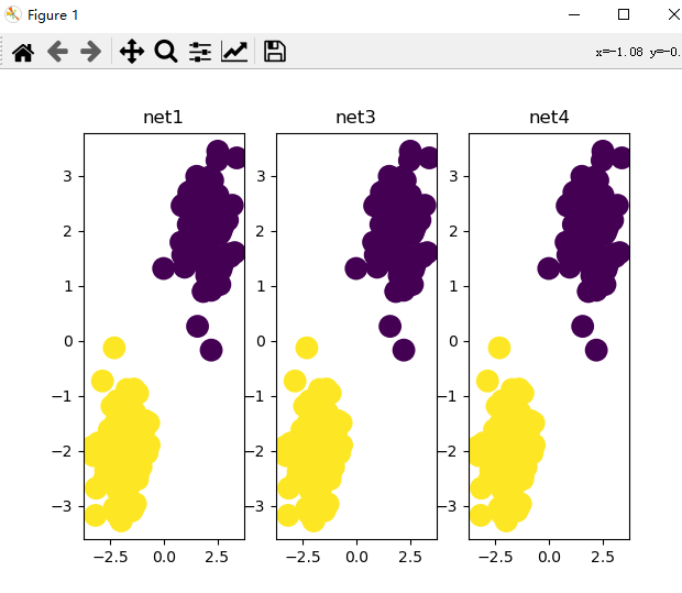
The first save torch.save() function saves the entire model and parameters. The second method only saves parameters. Similarly, there are two extraction methods, as above. Draw a picture and compare the results during training with those after saving and extraction.

 

3, Batch data training

import torch
import torch.utils.data as Data
BATCH_SIZE = 8
x = torch.linspace(1, 10, 10)
y = torch.linspace(10, 1, 10)
torch_dataset = Data.TensorDataset(x,y)
loader = Data.DataLoader(
    dataset=torch_dataset,
    batch_size=BATCH_SIZE,
    shuffle=True)
for epoch in range(3):
    for step, (batch_x, batch_y) in enumerate(loader):
        print('Epoch ', epoch, '| Step: ', step, '| batch x: ', batch_x.numpy(), '|batch y: ', batch_y.numpy())

Because the amount of data is too large to train all the data at one time, batch data is selected for training. As above, the torch.utils.data.TensorDataset() function constructs a data set, and the torch. Utils. Data. Dataloader() function constructs an iterator, batch_size is how many data are fetched each time.

4, Optimizer

opt_SGD         = torch.optim.SGD(net_SGD.parameters(), lr=LR)
opt_Momentum    = torch.optim.SGD(net_Momentum.parameters(), lr=LR, momentum=0.8)
opt_RMSprop     = torch.optim.RMSprop(net_RMSprop.parameters(), lr=LR, alpha=0.9)
opt_Adam        = torch.optim.Adam(net_Adam.parameters(), lr=LR, betas=(0.9, 0.99))

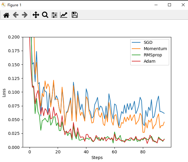
The above is the use method of the four optimizers. SGD is a random gradient descent, and the effect is the worst. The torch.optim.SGD(momentum =) parameter is the momentum optimizer, and the training speed of Adam optimizer is better than SGD. RMSprop is a combination of the two, as shown in the figure below, and the effect is better.

  5, Batch normalization

BN aims to standardize the scattered data. The data distribution will affect the training. If the input gap is too large, the output gap is too large, and the output may enter the insensitive part of the activation function after activation. Batch refers to batch data. BN is placed before the activation function to standardize all data to the sensitive area of the activation function. The process is to first calculate the average value of the data, then calculate the data variance, and then subtract the mean value from the data and divide the root sign of the variance to obtain the processed data. The data passes through a scaling coefficient to be trained to offset part of the negative optimization of the previous calculation.