Trigger word detection

Experimental topic

Trigger word detection

Experimental content

In this experiment, we understand how to apply deep learning to speech recognition. We will build speech data sets and implement trigger word detection algorithms (sometimes referred to as keyword detection or wake-up word detection). Trigger word detection is a technology that allows devices such as Amazon Alexa, Google Home, Apple Siri and Baidu DuerOS to wake up when they hear a word.

The trigger word for this exercise will be "activate". Every time we hear "activate", we will make a "Ding Dong" sound. At the end of this assignment, we can also record our own speech clips and let the algorithm trigger a prompt tone when it detects that we say "active".
In this assignment, we will learn:
- Building speech recognition projects
- Synthesize and process recordings to create training / development datasets
- Train the trigger word detection model and predict

Experimental steps

Import the relevant libraries required for the experiment

# Keras==2.2.5 tensorflow==1.15.0
!pip install pydub
import numpy as np
from pydub import AudioSegment
import random
import sys
import io
import os
import glob
import IPython
from td_utils import *
%matplotlib inline

1 - data synthesis: creating voice datasets

Firstly, we construct a data set for trigger word detection algorithm. Ideally, the voice dataset should be as close as possible to the application you want to run on. In this case, we want to detect the word "activation" in the working environment (library, home, office, open space...). Therefore, it is necessary to mix positive words ("activation") and negative words (random words other than activation) in different background sounds to create recordings.

1.1 - listening to data

In raw_ In the data directory, we can find a subset of the original audio files of positive words, negative words and background noise. We will use these audio file synthesis data sets to train the model. The "activate" directory contains positive examples of people saying the word "activate". The "negative" directory contains negative examples of random words that people say other than "activation". Each recording has a word. The "background" directory contains 10 seconds of background noise clips in different environments. We will use these three types of records (positive / negative / background) to create marker data sets. Below we can listen to the recording example:
```
IPython.display.Audio("./raw_data/activates/1.wav")
```

1.2 - from recording to spectrum

What is a real recording? Over time, the air pressure recorded by the microphone changes very little, and it is these small changes in air pressure that our ears will perceive as sound. We can think of the recording as a long string of numbers to measure the small changes in air pressure detected by the microphone. We will use audio sampled at 44100 Hz (or 44100 Hz). This means that the microphone gives us 44100 numbers per second. Therefore, a 10 second audio clip is represented by 441000 numbers (= $10 \times 44100 $).
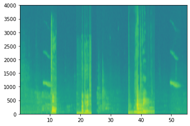
It is difficult to determine whether the word "activation" is said from this "original" representation of audio. In order to help our sequence model learn detection trigger words more easily, we will calculate the spectrum of audio. The spectrum diagram tells us how many different frequencies exist in the audio clip at a certain time. Next, we generate an audio spectrum:
```
x = graph_spectrogram("audio_examples/example_train.wav")
```
The results are as follows
The figure above shows the activity of each frequency (y-axis) on multiple time steps (x-axis).

**Figure 1 * *: spectrum diagram of audio recording, in which the color shows the occurrence (loudness) of different frequencies in audio at different time points. A green square indicates that a frequency is more active or more frequent (louder) in the audio clip; Blue squares indicate less active frequencies.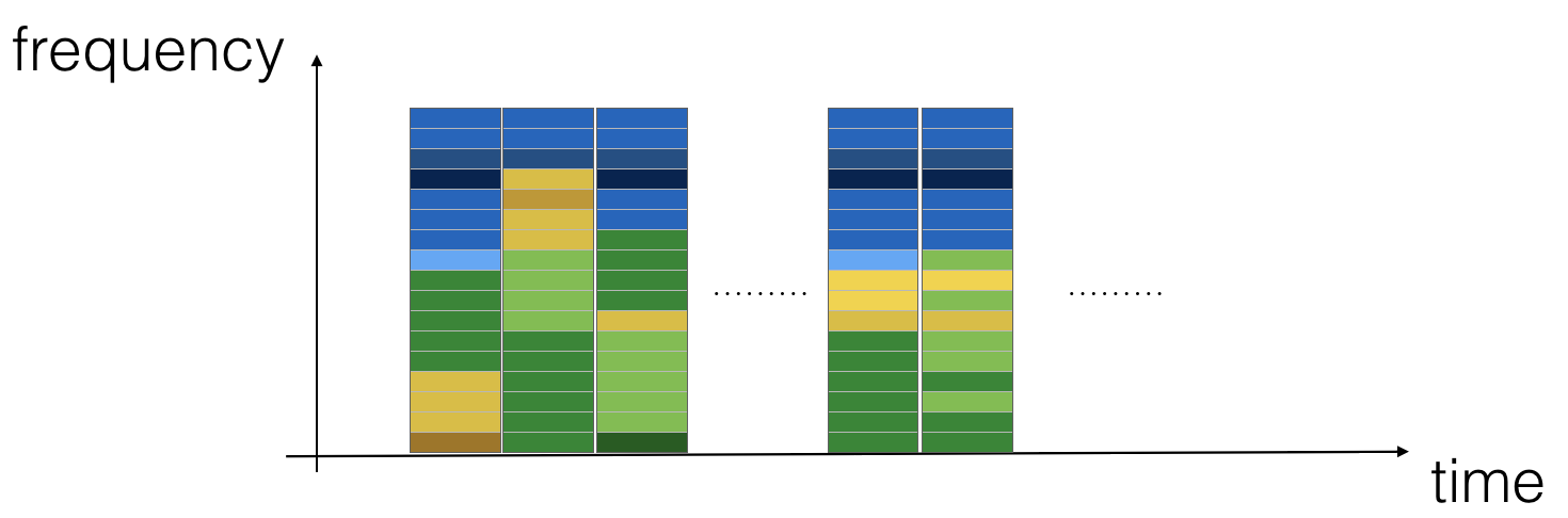

1.3 - generate a single training example

Because voice data is difficult to obtain and mark, we will use audio clips of activation, negatives and background to synthesize training data. Recording a large number of 10 second audio clips with random "activation" is very slow. Instead, it is easier to record a large number of positive and negative words and record background noise separately (or download background noise from free online resources).
To synthesize a single training example, we will:
- Select a random 10 second background audio clip
- Randomly insert 0-4 "active" audio clips in this 10 second clip
- Randomly insert 0-2 negative words into this 10 second clip
Since we have synthesized the word "activation" into the background clip, we know exactly when "activation" appears in the 10 second clip. As we will see later, this also enables the generation of tags y ⟨ t ⟩ y^{\langle t \rangle} y ⟨ t ⟩ becomes easier.

We will use the pydub package to manipulate audio. Pydub converts the original audio file into a list of pydub data structures (it's not important to understand the details here). Pydub uses 1ms as the discretization interval (1ms = 1/1000 second), which is why 10 second clips are always represented by 10000 steps.

# Load audio segments using pydub 
activates, negatives, backgrounds = load_raw_audio()

print("background len: " + str(len(backgrounds[0])))    # Should be 10,000, since it is a 10 sec clip
print("activate[0] len: " + str(len(activates[0])))     # Maybe around 1000, since an "activate" audio clip is usually around 1 sec (but varies a lot)
print("activate[1] len: " + str(len(activates[1])))     # Different "activate" clips can have different lengths 

# background len: 10000 
# activate[0] len: 721 
# activate[1] len: 731

Superimpose positive / negative words on the background:

Given a 10 second background clip and a short audio clip (positive or negative words), we need to "add" or "insert" the short audio clip of the word into the background. To ensure that audio clips inserted into the background do not overlap, we will track the time of previously inserted audio clips. We will insert clips with multiple positive / negative words on the background, and we don't want to insert "active" or random words where they overlap with another clip added earlier.
For clarity, when we insert a 1-second "activation" into a 10 second Cafe noise clip, we will eventually get a 10 second clip. It sounds like someone said "activation" in the cafe, and the "activation" is superimposed on the background Cafe noise without getting an 11 second clip. We will see how pydub performs this operation later.

Create labels while superimposing:

Remember the label y ⟨ t ⟩ y^{\langle t \rangle} y ⟨ t ⟩ indicates whether someone has just finished "activate". Given a background clip, we can provide all t t t initialization y ⟨ t ⟩ = 0 y^{\langle t \rangle}=0 y ⟨ t ⟩ = 0 because the clip does not contain any activation.
It will also be updated when we insert or overwrite the active clip y ⟨ t ⟩ y^{\langle t \rangle} y ⟨ t ⟩ so that 50 steps of output now have target tag 1. We will train GRU to detect when someone has finished saying "activate". For example, suppose a composite "active" clip ends at the 5-second mark in 10 second audio -- exactly half the clip. Think back T y = 1375 T_y = 1375 Ty = 1375, so the time step $687 = $int (1375 * 0.5) corresponds to the time when the audio is entered for 5 seconds. Therefore, we will set y ⟨ 688 ⟩ = 1 y^{\langle 688 \rangle} = 1 y⟨688⟩=1. In addition, if GRU detects "activation" in a short time after this time, we will be very satisfied, so we will actually label it y ⟨ t ⟩ y^{\langle t \rangle} Set * * 50 consecutive values * * of y ⟨ t ⟩ to 1. Specifically, we have y ⟨ 688 ⟩ = y ⟨ 689 ⟩ = ⋯ = y ⟨ 737 ⟩ = 1 y^{\langle 688 \rangle} = y^{\langle 689 \rangle} = \cdots = y^{\langle 737 \rangle} = 1 y⟨688⟩=y⟨689⟩=⋯=y⟨737⟩=1
This is another reason for synthesizing training data: these tags are generated as described above y ⟨ t ⟩ y^{\langle t \rangle} y ⟨ t ⟩ is relatively simple. In contrast, if we record 10 seconds of audio on the microphone, it will be very time-consuming for a person to listen to it and mark it accurately manually when the "activation" is completed.
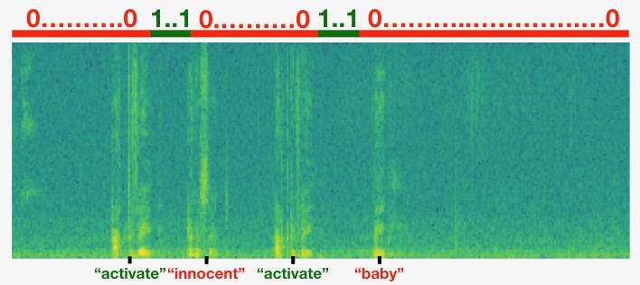
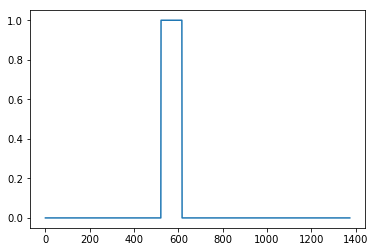
Below is a description label y ⟨ t ⟩ y^{\langle t \rangle} For the graph of y ⟨ t ⟩ we inserted clips of "activation", "innocent", "activation" and "baby". Note that the positive label "1" is associated with only positive words.

**Figure 2**

To implement the training set synthesis process, we will use the following auxiliary functions. All these functions will use a discretization interval of 1ms, so 10 seconds of audio is always discretized into 10000 steps.
- 1.get_random_time_segment(segment_ms) gets a random time period in our background audio
- 2.is_overlapping(segment_time, existing_segments) checks whether the time period overlaps with the existing segment
- 3.insert_audio_clip(background, audio_clip, existing_times) uses get_random_time_segment and is_overlapping randomly inserts an audio clip into our background audio
- 4.insert_ones(y, segment_end_ms) inserts 1 into our label vector y after the word "activate"

Function * * get_random_time_segment(segment_ms) * * returns a random time period in which we can insert audio clips with a duration of "segment_ms".

def get_random_time_segment(segment_ms):
    """
    Gets a random time segment of duration segment_ms in a 10,000 ms audio clip.
    
    Arguments:
    segment_ms -- the duration of the audio clip in ms ("ms" stands for "milliseconds")
    
    Returns:
    segment_time -- a tuple of (segment_start, segment_end) in ms
    """
    
    segment_start = np.random.randint(low=0, high=10000-segment_ms)   # Make sure segment doesn't run past the 10sec background 
    segment_end = segment_start + segment_ms - 1
    print("segment_time is [%d,%d]"%(segment_start,segment_end))
    return (segment_start, segment_end)

Next, suppose we have inserted audio clips in segments (1000, 1800) and (34004500). That is, the first segment starts at step 1000 and ends at step 1800. Now, if we consider inserting a new audio clip at (30003600), does this overlap with one of the previously inserted clips? In this case, (30003600) and (34004500) overlap, so we should decide not to insert clips here.
For the purpose of this function, (100200) and (200250) are defined as overlapping because they overlap at time step 200. However, (100199) and (200250) do not overlap.

Exercise: function is_overlapping(segment_time, existing_segments) to check whether the new time period overlaps any previous period. We will need to perform 2 steps:

1. Create a "False" flag. If we find overlap, we will set it to "True" later.
2. Cycle previous_ Start and end times of segments. Compare these times with the start and end times of the segment. If there is overlap, set the flag defined in (1) to True.

# GRADED FUNCTION: is_overlapping

def is_overlapping(segment_time, previous_segments):
    """
    Checks if the time of a segment overlaps with the times of existing segments.
    
    Arguments:
    segment_time -- a tuple of (segment_start, segment_end) for the new segment
    previous_segments -- a list of tuples of (segment_start, segment_end) for the existing segments
    
    Returns:
    True if the time segment overlaps with any of the existing segments, False otherwise
    """
    
    segment_start, segment_end = segment_time
    
    ### START CODE HERE ### (≈ 4 line)
    # Step 1: Initialize overlap as a "False" flag. (≈ 1 line)
    overlap = False
    
    # Step 2: loop over the previous_segments start and end times.
    # Compare start/end times and set the flag to True if there is an overlap (≈ 3 lines)
    for previous_start, previous_end in previous_segments:
        if segment_start<=previous_end and segment_end>=previous_start:
            overlap = True
    ### END CODE HERE ###

    return overlap

The test results are shown as follows

overlap1 = is_overlapping((950, 1430), [(2000, 2550), (260, 949)])
overlap2 = is_overlapping((2305, 2950), [(824, 1532), (1900, 2305), (3424, 3656)])
print("Overlap 1 = ", overlap1) # False
print("Overlap 2 = ", overlap2) # True

Now, let's use the previous auxiliary function to randomly insert a new audio clip in the background of 10 seconds, but make sure that any newly inserted clip does not overlap the previous clip.

Exercise: implementing insert_audio_clip() superimposes the audio clip on the background 10 second clip. We will need to perform four steps:

1. Gets the random time period of the correct duration in milliseconds.
1. Make sure that the time period does not overlap any previous time periods. If there is overlap, return to step 1 and select a new time period.
1. Add a new time period to the list of existing time periods to track all the time periods we inserted.
1. Use pydub to overlay the audio clip on the background.

# GRADED FUNCTION: insert_audio_clip

def insert_audio_clip(background, audio_clip, previous_segments):
    """
    Insert a new audio segment over the background noise at a random time step, ensuring that the 
    audio segment does not overlap with existing segments.
    
    Arguments:
    background -- a 10 second background audio recording.  
    audio_clip -- the audio clip to be inserted/overlaid. 
    previous_segments -- times where audio segments have already been placed
    
    Returns:
    new_background -- the updated background audio
    """
    
    # Get the duration of the audio clip in ms
    segment_ms = len(audio_clip)
    
    ### START CODE HERE ### 
    # Step 1: Use one of the helper functions to pick a random time segment onto which to insert 
    # the new audio clip. (≈ 1 line)
    segment_time = get_random_time_segment(segment_ms)
    
    # Step 2: Check if the new segment_time overlaps with one of the previous_segments. If so, keep 
    # picking new segment_time at random until it doesn't overlap. (≈ 2 lines)
    while is_overlapping(segment_time,previous_segments):
        segment_time = get_random_time_segment(segment_ms)

    # Step 3: Add the new segment_time to the list of previous_segments (≈ 1 line)
    previous_segments.append(segment_time)
    ### END CODE HERE ###
    
    # Step 4: Superpose audio segment and background
    new_background = background.overlay(audio_clip, position = segment_time[0])
    
    return new_background, segment_time

The test is carried out below, and the results are shown as follows

np.random.seed(5)
audio_clip, segment_time = insert_audio_clip(backgrounds[0], activates[0], [(3790, 4400)])
audio_clip.export("insert_test.wav", format="wav")
print("Segment Time: ", segment_time)
IPython.display.Audio("insert_test.wav")

# Segment Time:  (2915, 3635)

Finally, implement the code to update the tag y ⟨ t ⟩ y^{\langle t \rangle} Y ⟨ t ⟩ suppose we just inserted an "activation". In the following code, y is a (11375) dimensional vector because T y = 1375 T_y = 1375 Ty=1375.
If "active" is in the time step t t t end, set y ⟨ t + 1 ⟩ = 1 y^{\langle t+1 \rangle} = 1 Y ⟨ t+1 ⟩ = 1 and up to 49 additional continuous values. However, make sure you don't go beyond the end of the array and try to update y[0][1375], because the valid indexes are y[0][0] to y[0][1374] T y = 1375 T_y = 1375 Ty=1375. Therefore, if "activation" ends in step 1370, we will only get y[0][1371] = y[0][1372] = y[0][1373] = y[0][1374] = 1

Exercise: implementing insert_ones(), you can use the for loop. If a segment is represented by segment_end_ms ends (using 10000 steps of discretization) and converts it to output y y Index of y (use) 1375 1375 1375 steps (discretization), we will use the following formula:
segment_end_y = int(segment_end_ms * Ty / 10000.0)

# GRADED FUNCTION: insert_ones

def insert_ones(y, segment_end_ms):
    """
    Update the label vector y. The labels of the 50 output steps strictly after the end of the segment 
    should be set to 1. By strictly we mean that the label of segment_end_y should be 0 while, the
    50 followinf labels should be ones.
    
    
    Arguments:
    y -- numpy array of shape (1, Ty), the labels of the training example
    segment_end_ms -- the end time of the segment in ms
    
    Returns:
    y -- updated labels
    """
    
    # duration of the background (in terms of spectrogram time-steps)
    segment_end_y = int(segment_end_ms * Ty / 10000.0)
    
    # Add 1 to the correct index in the background label (y)
    ### START CODE HERE ### (≈ 3 lines)
    for i in range(segment_end_y + 1, segment_end_y + 1 + 50):
        if i < Ty:
            y[0, i] = 1
    ### END CODE HERE ###
    
    return y

Let's test, and the test results are as follows

arr1 = insert_ones(np.zeros((1, Ty)), 9700)
plt.plot(insert_ones(arr1, 4251)[0,:])
print("sanity checks:", arr1[0][1333], arr1[0][634], arr1[0][635])

Finally, we can use insert_audio_clip and insert_ One creates a new training example.

Exercise: implementing create_training_example(), we need to perform the following steps:

1. Label vector y y y is initialized to a zero sum shape ( 1 , T y ) (1, T_y) numpy array composed of (1,Ty).
2. Initialize the existing segment set as an empty list.
3. Randomly select 0 to 4 "active" audio clips and insert them into the 10 second clip. Also in the label vector y y Insert the label in the correct position in y.
4. Randomly select 0 to 2 negative audio and insert 10sec segments.

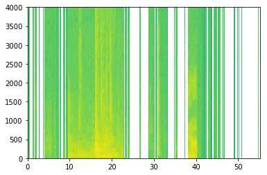
# GRADED FUNCTION: create_training_example

def create_training_example(background, activates, negatives):
    """
    Creates a training example with a given background, activates, and negatives.
    
    Arguments:
    background -- a 10 second background audio recording
    activates -- a list of audio segments of the word "activate"
    negatives -- a list of audio segments of random words that are not "activate"
    
    Returns:
    x -- the spectrogram of the training example
    y -- the label at each time step of the spectrogram
    """
    
    # Set the random seed
    np.random.seed(18)
    
    # Make background quieter
    background = background - 20

    ### START CODE HERE ###
    # Step 1: Initialize y (label vector) of zeros (≈ 1 line)
    y = np.zeros((1, Ty))

    # Step 2: Initialize segment times as empty list (≈ 1 line)
    previous_segments = []
    ### END CODE HERE ###
    
    # Select 0-4 random "activate" audio clips from the entire list of "activates" recordings
    number_of_activates = np.random.randint(0, 5)
    random_indices = np.random.randint(len(activates), size=number_of_activates)
    random_activates = [activates[i] for i in random_indices]
    
    ### START CODE HERE ### (≈ 3 lines)
    # Step 3: Loop over randomly selected "activate" clips and insert in background
    for random_activate in random_activates:
        # Insert the audio clip on the background
        background, segment_time = insert_audio_clip(background,random_activate,previous_segments)
        # Retrieve segment_start and segment_end from segment_time
        segment_start, segment_end = segment_time
        # Insert labels in "y"
        y = insert_ones(y,segment_end_ms=segment_end)
    ### END CODE HERE ###

    # Select 0-2 random negatives audio recordings from the entire list of "negatives" recordings
    number_of_negatives = np.random.randint(0, 3)
    random_indices = np.random.randint(len(negatives), size=number_of_negatives)
    random_negatives = [negatives[i] for i in random_indices]

    ### START CODE HERE ### (≈ 2 lines)
    # Step 4: Loop over randomly selected negative clips and insert in background
    for random_negative in random_negatives:
        # Insert the audio clip on the background 
        background, _ = insert_audio_clip(background,random_negative,previous_segments)
    ### END CODE HERE ###
    
    # Standardize the volume of the audio clip 
    background = match_target_amplitude(background, -20.0)

    # Export new training example 
    file_handle = background.export("train" + ".wav", format="wav")
    print("File (train.wav) was saved in your directory.")
    
    # Get and plot spectrogram of the new recording (background with superposition of positive and negatives)
    x = graph_spectrogram("train.wav")
    
    return x, y

x, y = create_training_example(backgrounds[0], activates, negatives)

The results are as follows

Now we can listen to the training example created and compare it with the spectrum generated above.
```
IPython.display.Audio("train.wav")
IPython.display.Audio("audio_examples/train_reference.wav")
```
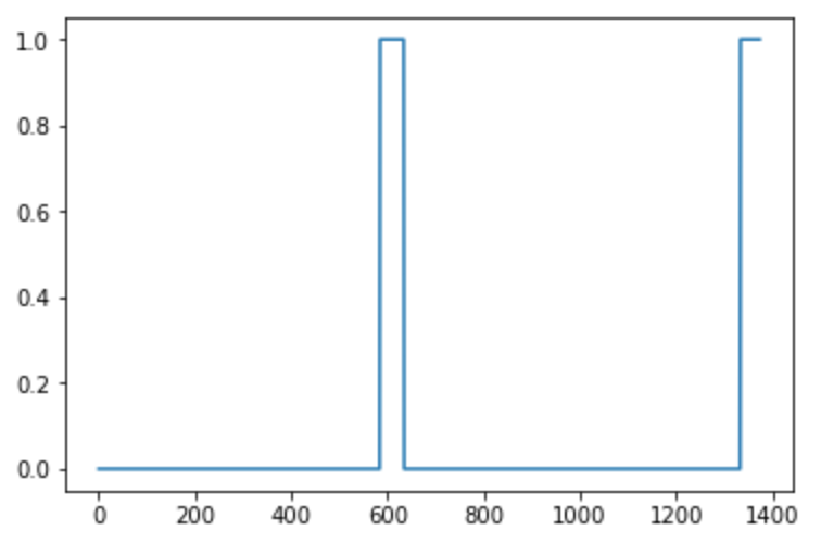
Finally, we can draw relevant labels for the generated training examples as follows
```
plt.plot(y[0])
```

1.4 - complete training set

Now that we have implemented the code required to generate a single training example, we use this process to generate a large training set. To save time, we have generated a set of training examples to call directly
```
# Load preprocessed training examples
X = np.load("./XY_train/X.npy")
Y = np.load("./XY_train/Y.npy")
```

1.5 - development set

To test our model, we documented a development set of 25 examples. Although our training data is synthetic, we want to create a development set with the same distribution as the actual input. So we recorded 25 10 second audio clips that people said "activate" and other random words and marked them manually. This follows the principle described earlier, that is, we should create a development set as similar to the distribution of the test set as possible, which is why our development set uses real audio instead of synthetic audio. Next, we load the preprocessed development set example
```
# Load preprocessed dev set examples
X_dev = np.load("./XY_dev/X_dev.npy")
Y_dev = np.load("./XY_dev/Y_dev.npy")
```

2 - model

Now that we have built a data set, let's write and train the trigger word detection model!

The model will use one-dimensional convolution layer, GRU layer and dense layer. Let's load packages that allow these layers to be used in Keras

from keras.callbacks import ModelCheckpoint
from keras.models import Model, load_model, Sequential
from keras.layers import Dense, Activation, Dropout, Input, Masking, TimeDistributed, LSTM, Conv1D
from keras.layers import GRU, Bidirectional, BatchNormalization, Reshape
from keras.optimizers import Adam

2.1 - building models

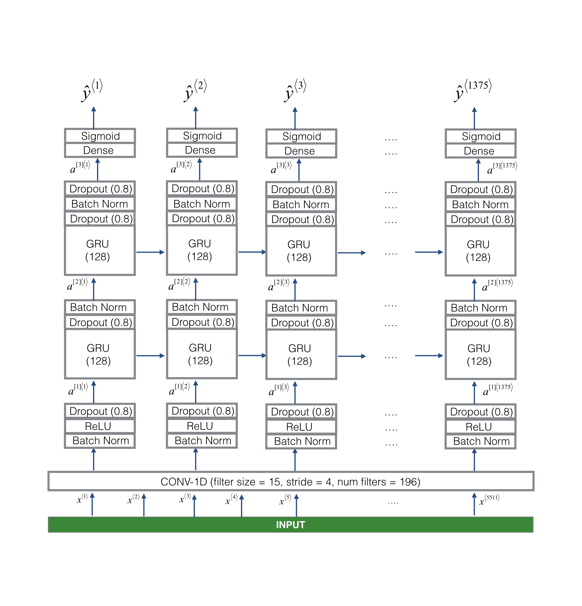
This is the architecture we will use
A key step of the model is the one-dimensional convolution step (near the bottom of Figure 3). It inputs 5511 step spectrum and outputs 1375 step output, and then after multi-layer further processing, the final spectrum is obtained T y = 1375 T_y=1375 Ty = 1375 step output. The function of this layer is similar to 2D convolution, that is, extracting low-level features and then generating smaller dimensional output.
In terms of calculation, one-dimensional convolution also helps to accelerate the model, because GRU only needs to process 1375 time steps instead of 5511 time steps. The two GRU layers read the input sequence from left to right, and then finally use the dense + sigmoid layer pair y ⟨ t ⟩ y^{\langle t \rangle} y ⟨ t ⟩ for prediction. because y y y is the binary value (0 or 1). At the last layer, we use sigmoid output to estimate the chance of output as 1, which corresponds to the user who just said "activated".
Note that we use unidirectional RNN instead of bidirectional RNN. This is very important for trigger word detection, because we want to detect it almost immediately after the trigger word is spoken. If we use bidirectional RNN, we will have to wait for the entire 10 seconds of audio to be recorded before we can judge whether "active" is said in the first second of the audio clip.
The implementation of the model can be divided into four steps:

Step 1: the CONV layer is implemented using Conv1D(). There are 196 filters with a filter size of 15 (kernel_size=15) and a step size of 4. [ See documentation.]

Step 2: the first GRU layer. To generate a GRU layer, you can use:
X = GRU (unit = 128, return_sequences = True) (X)
Setting return_sequences=True ensures that the hidden state of all Grus is fed to the next layer. Remember to follow this in the Dropout and BatchNorm layers.

Step 3: the second GRU layer. This is similar to the previous GRU layer (remember to use return_sequences=True), but there is an additional dropout layer.

Step 4: create a dense layer with time distribution as follows:
X = TimeDistributed(Dense(1, activation = "sigmoid"))(X)
This creates a dense layer, followed by a sigmoid, so that the parameters used by the dense layer are the same for each time step[ See documentation. ]

Exercise: Implement model(), the architecture is shown in the figure above, and the implementation code is as follows:

# GRADED FUNCTION: model

def model(input_shape):
    """
    Function creating the model's graph in Keras.
    
    Argument:
    input_shape -- shape of the model's input data (using Keras conventions)

    Returns:
    model -- Keras model instance
    """
    
    X_input = Input(shape = input_shape)
    
    ### START CODE HERE ###
    
    # Step 1: CONV layer (≈4 lines)
    X = Conv1D(filters=196, kernel_size=15, strides=4)(X_input)     # CONV1D
    X = BatchNormalization()(X)                                     # Batch normalization
    X = Activation('relu')(X)                                       # ReLu activation
    X = Dropout(0.8)(X)                                             # dropout (use 0.8)

    # Step 2: First GRU Layer (≈4 lines)
    X = GRU(units=128, return_sequences=True)(X)                    # GRU (use 128 units and return the sequences)
    X = Dropout(0.8)(X)                                             # dropout (use 0.8)
    X = BatchNormalization()(X)                                     # Batch normalization
    
    # Step 3: Second GRU Layer (≈4 lines)
    X = GRU(units=128, return_sequences=True)(X)                    # GRU (use 128 units and return the sequences)
    X = Dropout(0.8)(X)                                             # dropout (use 0.8)
    X = BatchNormalization()(X)                                     # Batch normalization
    X = Dropout(0.8)(X)                                             # dropout (use 0.8)
    
    # Step 4: Time-distributed dense layer (≈1 line)
    X = TimeDistributed(Dense(1, activation = "sigmoid"))(X)        # time distributed  (sigmoid)

    ### END CODE HERE ###

    model = Model(inputs = X_input, outputs = X)
    
    return model

Generation model

model = model(input_shape = (Tx, n_freq))

Let's print the model summary to track the shape
```
model.summary()
```
The output shape of the network is (None, 1375, 1) and the input shape is (None, 5511, 101). Conv1D reduces the number of steps of the spectrum from 5511 to 1375.

2.2 - Fit the model

Trigger word detection takes a long time to train. In order to save time, we have trained the model for about 3 hours on the GPU using the above architecture and a large training set of about 4000 examples. Let's load the model
```
model = load_model('./models/tr_model.h5')
```
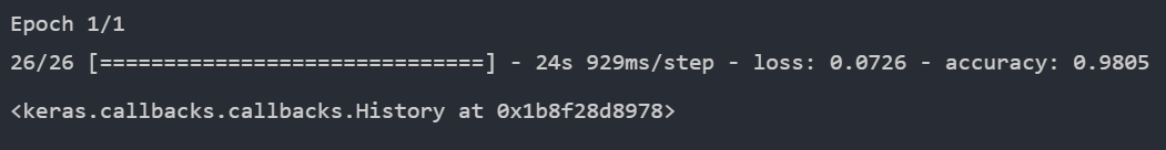
We can further train the model using Adam optimizer and binary cross entropy loss, as shown below. This will run quickly because we train for only one period and use a small training set of 26 examples.
```
opt = Adam(lr=0.0001, beta_1=0.9, beta_2=0.999, decay=0.01)
model.compile(loss='binary_crossentropy', optimizer=opt, metrics=["accuracy"])
model.fit(X, Y, batch_size = 5, epochs=1)
```
You can see the training process as follows

2.3 - Test Model

Finally, let's see how your model performs on the development set

loss, acc = model.evaluate(X_dev, Y_dev)
print("Dev set accuracy = ", acc)

# Dev set accuracy =  0.9451636075973511

This looks good! However, accuracy is not an important indicator of this task, because the label is seriously biased towards 0, so the neural network that only outputs 0 will obtain an accuracy of slightly higher than 90%. We can define more useful indicators, such as F1 score or Precision/Recall. But let's not worry here, but just look at how the model does it by experience.

3 - make predictions

Now that we have built a working model for trigger word detection, let's use it to predict. This code fragment runs audio over the network (saved in wav file)

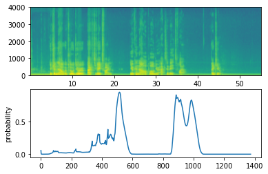
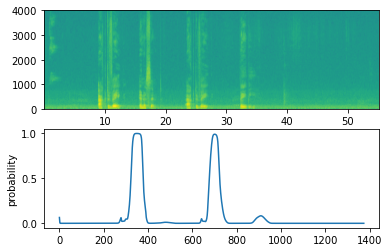
def detect_triggerword(filename):
    plt.subplot(2, 1, 1)

    x = graph_spectrogram(filename)
    # the spectogram outputs (freqs, Tx) and we want (Tx, freqs) to input into the model
    x  = x.swapaxes(0,1)
    x = np.expand_dims(x, axis=0)
    predictions = model.predict(x)
    
    plt.subplot(2, 1, 2)
    plt.plot(predictions[0,:,0])
    plt.ylabel('probability')
    plt.show()
    return predictions

Once we estimate the probability of detecting the word "active" in each output step, you can trigger the "bell" sound playback when the probability is higher than a certain threshold. In addition, after saying "active", for many consecutive values, y ⟨ t ⟩ y^{\langle t \rangle} y ⟨ t ⟩ may be close to 1, but we only want to sound once. So we insert a prompt tone at most every 75 output steps. This will help prevent us from inserting two bells for a single "active" instance (which is similar to non maximum suppression in computer vision)

chime_file = "audio_examples/chime.wav"
def chime_on_activate(filename, predictions, threshold):
    audio_clip = AudioSegment.from_wav(filename)
    chime = AudioSegment.from_wav(chime_file)
    Ty = predictions.shape[1]
    # Step 1: Initialize the number of consecutive output steps to 0
    consecutive_timesteps = 0
    # Step 2: Loop over the output steps in the y
    for i in range(Ty):
        # Step 3: Increment consecutive output steps
        consecutive_timesteps += 1
        # Step 4: If prediction is higher than the threshold and more than 75 consecutive output steps have passed
        if predictions[0,i,0] > threshold and consecutive_timesteps > 75:
            # Step 5: Superpose audio and background using pydub
            audio_clip = audio_clip.overlay(chime, position = ((i / Ty) * audio_clip.duration_seconds)*1000)
            # Step 6: Reset consecutive output steps to 0
            consecutive_timesteps = 0
        
    audio_clip.export("chime_output.wav", format='wav')

3.1 - Test on dev examples

Let's explore how our model handles two invisible audio clips from the development set. Let's listen to the two development set clips first.
```
IPython.display.Audio("./raw_data/dev/1.wav")
IPython.display.Audio("./raw_data/dev/2.wav")
```

Now let's run the model on these audio clips to see if it adds a prompt tone after "activation"!

filename = "./raw_data/dev/1.wav"
prediction = detect_triggerword(filename)
chime_on_activate(filename, prediction, 0.5)
IPython.display.Audio("./chime_output.wav")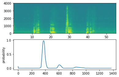

filename  = "./raw_data/dev/2.wav"
prediction = detect_triggerword(filename)
chime_on_activate(filename, prediction, 0.5)
IPython.display.Audio("./chime_output.wav")

4 - try your own example

Record a 10 second audio clip, let you say the word "activate" and other random words, and then upload it to the Coursera center as "myaudio.wav". Be sure to upload the audio as a wav file. If your audio is in a different format (such as mp3) Recording, you can find free software on the Internet to convert it to wav. If your recording is not 10 seconds, the following code will trim or fill it as needed to make it 10 seconds.
```
# Preprocess the audio to the correct format
def preprocess_audio(filename):
    # Trim or pad audio segment to 10000ms
    padding = AudioSegment.silent(duration=10000)
    segment = AudioSegment.from_wav(filename)[:10000]
    segment = padding.overlay(segment)
    # Set frame rate to 44100
    segment = segment.set_frame_rate(44100)
    # Export as wav
    segment.export(filename, format='wav')
```

After uploading the audio file to Coursera, put the file path in the following variable.

your_filename = "audio_examples/my_audio.wav"
preprocess_audio(your_filename)
IPython.display.Audio(your_filename) # listen to the audio you uploaded

Finally, use the model to predict when to say "active" in a 10 second audio clip and trigger a prompt tone. If the beep is not added correctly, try adjusting the chime_threshold.
```
chime_threshold = 0.5
prediction = detect_triggerword(your_filename)
chime_on_activate(your_filename, prediction, chime_threshold)
IPython.display.Audio("./chime_output.wav")
```

Keywords: Python Deep Learning Deeplearning

Added by activeserver on Thu, 09 Dec 2021 12:27:57 +0200

Programming VIP