Deep learning
Basic knowledge and various network structurespreface
It is very important to learn a good framework for in-depth learning. Now the mainstream is pytoch and tf. Let's learn pytoch together today ! [insert picture description here]( https://img-blog.csdnimg.cn/25238d12cb8641b8bc38171559ab41e9.jpg#pic_center)1, Basic data: Tensor
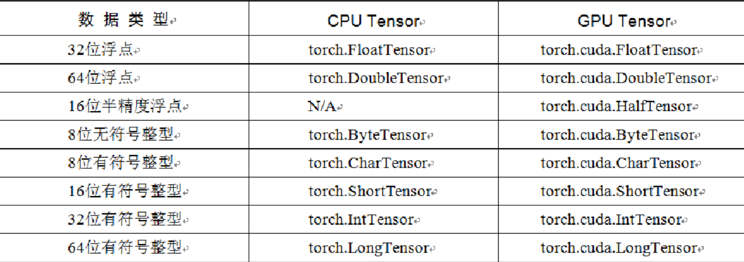
Tensor, or tensor, is the basic operation object in PyTorch and can be regarded as a multidimensional matrix containing a single data type element. From the perspective of usage, tensor is very similar to NumPy's darrys, and can be freely converted to each other, but tensor also supports GPU acceleration.
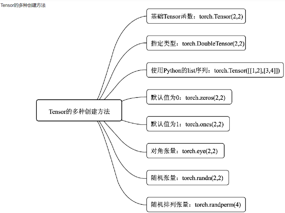
1.1 creation of tensor
1.2 torch.FloatTensor
torch.FloatTensor is used to generate tensors with floating-point data type and pass them to torch The parameter of floattensor can be a list or a dimension value.
import torch
a = torch.FloatTensor(2,3)
b = torch.FloatTensor([2,3,4,5])
a,b
The results are:
(tensor([[1.0561e-38, 1.0102e-38, 9.6429e-39],
         [8.4490e-39, 9.6429e-39, 9.1837e-39]]),
 tensor([2., 3., 4., 5.]))
1.3 torch.IntTensor
torch.IntTensor is used to generate Tensor with integer data type and pass it to torch The parameter of inttensor can be a list or a dimension value.
import torch
a = torch.FloatTensor(2,3)
b = torch.FloatTensor([2,3,4,5])
a,b
import torch
a = torch.rand(2,3)
a
Get:
tensor([[0.5625, 0.5815, 0.8221],
        [0.3589, 0.4180, 0.2158]])
1.4 torch.randn
It is used to generate random Tensor with floating-point data type and dimension specified, and numpy used in numpy The random number generated by randn is similar. The value of the randomly generated floating-point number satisfies the normal distribution with mean value of 0 and variance of 1.
import torch
a = torch.randn(2,3)
a
Get:
tensor([[-0.0067, -0.0707, -0.6682],
        [ 0.8141,  1.1436,  0.5963]])
1.5 torch.range
torch.range is used to generate Tensor with floating-point data type and start range and end range, so it is passed to torch Range has three parameters: start value, end value and step size. The step size is used to specify the data interval of each step from the start value to the end value.
import torch
a = torch.range(1,20,2)
a
Get:
tensor([ 1., 3., 5., 7., 9., 11., 13., 15., 17., 19.])
1.6 torch.zeros/ones/empty
torch.zeros is used to generate tensors with floating-point data type and dimension specified, but the element values in tensors of this floating-point type are all 0.
torch.ones generates an array of all 1.
torch.empty creates an uninitialized tensor whose size is determined by size. Size: defines the shape of the tensor, which can be a list or a tuple
import torch
a = torch.zeros(2,3)
a
Get:
tensor([[0., 0., 0.],
        [0., 0., 0.]])
2, Tensor's operation
2.1 torch.abs
Pass parameters to torch ABS returns the absolute value of the input parameter as the output. The input parameter must be a variable of Tensor data type, such as:
import torch
a = torch.randn(2,3)
a
The result a is:
tensor([[ 0.0948,  0.0530, -0.0986],
        [ 1.8926, -2.0569,  1.6617]])
abs treatment for a:
b = torch.abs(a)
b
Get:
tensor([[0.0948, 0.0530, 0.0986],
        [1.8926, 2.0569, 1.6617]])
2.2 torch.add
Pass parameters to torch Add returns the summation result of the input parameters as output. The input parameters can be all variables of Tensor data type, one variable of Tensor data type and the other scalar.
import torch
a = torch.randn(2,3)
a
#tensor([[-0.1146, -0.3282, -0.2517],
#        [-0.2474,  0.8323, -0.9292]])
b = torch.randn(2,3)
b
#tensor([[ 0.9526,  1.5841, -3.2665],
#        [-0.4831,  0.9259, -0.5054]])
c = torch.add(a,b)
c
Output c:
tensor([[ 0.8379,  1.2559, -3.5182],
        [-0.7305,  1.7582, -1.4346]])
Take another look:
d = torch.randn(2,3)
d
#Here we get d:
#tensor([[ 0.1473,  0.7631, -0.1953],
#        [-0.2796, -0.7265,  0.7142]])
We add d to a scalar 10:
e = torch.add(d,10)
e
Get:
tensor([[10.1473, 10.7631,  9.8047],
        [ 9.7204,  9.2735, 10.7142]])
2.3 torch.clamp
torch.clamp cuts the input parameters according to the user-defined range, and finally takes the result of parameter cutting as the output. Therefore, there are three input parameters, namely, the variable of Tensor data type to be cut, the upper boundary of cutting and the lower boundary of cutting, The specific clipping process is as follows: each element in the variable is compared with the values of the clipped upper boundary and the clipped lower boundary respectively. If the value of the element is less than the value of the clipped lower boundary, the element is rewritten as the value of the clipped lower boundary; Similarly, if the value of an element is greater than the value of the clipped upper boundary, the element is rewritten to the value of the clipped upper boundary. Let's look directly at the example:
a = torch.randn(2,3)
a
#We get a as:
#tensor([[-1.4049,  1.0336,  1.2820],
#        [ 0.7610, -1.7475,  0.2414]])
We clap b:
b = torch.clamp(a,-0.1,0.1)
b
#We get b as:
#tensor([[-0.1000,  0.1000,  0.1000],
#        [ 0.1000, -0.1000,  0.1000]])
2.4 torch.div
torch.div is the parameter passed to torch After div, the quotient result of the input parameters is returned as the output. Similarly, all the parameters involved in the operation can be variables of Tensor data type, or a combination of variables of Tensor data type and scalar. Let's look at examples
a = torch.randn(2,3)
a
#We get a as:
#tensor([[ 0.6276,  0.6397, -0.0762],
#        [-0.4193, -0.5528,  1.5192]])
b = torch.randn(2,3)
b
#We get b as:
#tensor([[ 0.9219,  0.2120,  0.1155],
#        [ 1.1086, -1.1442,  0.2999]])
Perform div operation on a and B
c = torch.div(a,b)
c
#Get c:
#tensor([[ 0.6808,  3.0173, -0.6602],
#        [-0.3782,  0.4831,  5.0657]])
2.5 torch.pow
torch.pow: pass parameters to torch POW returns the exponentiation result of the input parameter as the output. All the parameters involved in the operation can be variables of Tensor data type or a combination of variables of Tensor data type and scalar.
a = torch.randn(2,3)
a
#We get a as:
#tensor([[ 0.3896, -0.1475,  0.1104],
#        [-0.6908, -0.0472, -1.5310]])
Square a
b = torch.pow(a,2)
b
#We get b as:
#tensor([[1.5181e-01, 2.1767e-02, 1.2196e-02],
#        [4.7722e-01, 2.2276e-03, 2.3441e+00]])
2.6 torch.mm
torch.mm: pass parameters to torch Mm returns the quadrature result of the input parameter as output, but this quadrature method is the same as the previous torch Mul operation is different, torch Mm uses the multiplication rules between matrices for calculation, so the passed in parameters will be treated as a matrix, and the dimension of the parameters must naturally meet the preconditions of matrix multiplication, that is, the number of rows of the previous matrix must be equal to the number of columns of the latter matrix
Let's take an example:
a = torch.randn(2,3)
a
#We get a as:
#tensor([[ 0.1057,  0.0104, -0.1547],
#        [ 0.5010, -0.0735,  0.4067]])
b = torch.randn(2,3)
b
#We get b as:
#tensor([[ 1.1971, -1.4010,  1.1277],
#        [-0.3076,  0.9171,  1.9135]])
Then we use the generated a and B to perform matrix multiplication:
c = torch.mm(a,b.T)
c
#tensor([[-0.0625, -0.3190],
#        [ 1.1613,  0.5567]])
2.7 torch.mv
Pass parameters to torch MV returns the quadrature result of the input parameter as the output, torch MV is calculated by using the multiplication rules between matrix and vector. The first parameter passed in represents the matrix and the second parameter represents the vector. The sequence cannot be reversed.
Let's take an example:
a = torch.randn(2,3)
a
#We get a as:
#tensor([[ 1.0909, -1.1679,  0.3161],
#        [-0.8952, -2.1351, -0.9667]])
b = torch.randn(3)
b
#We get b as:
#tensor([-1.4689,  1.6197,  0.7209])
Then we use the generated a and B to perform matrix multiplication:
c = torch.mv(a,b)
c
#tensor([-3.2663, -2.8402])
3, Neural network toolbox torch nn
torch. Although Autograd library realizes automatic derivation and gradient back propagation, if we want to complete the training of a model, we still need the automatic updating of handwritten parameters and the control of training process, which is not convenient enough. To this end, PyTorch further provides a more integrated modular interface torch NN, which is built on Autograd and provides a series of functions such as network module, optimizer and initialization strategy.
3.1 nn.Module class
nn.Module is a neural network class provided by PyTorch, which implements the definition of each layer of the network and the forward calculation and back propagation mechanism. In practical use, if you want to implement a neural network, you only need to inherit NN Module, define the model structure and parameters during initialization, and write the network forward process in the function forward().
1.nn.Parameter function
2. forward() function and back propagation
3. Nesting of multiple modules
4.nn.Module and NN Functional library
5.nn.Sequential() module
#Use torch here NN implement an MLP
from torch import nn

class MLP(nn.Module):
    def __init__(self, in_dim, hid_dim1, hid_dim2, out_dim):
        super(MLP, self).__init__()
        self.layer = nn.Sequential(
          nn.Linear(in_dim, hid_dim1),
          nn.ReLU(),
          nn.Linear(hid_dim1, hid_dim2),
          nn.ReLU(),
          nn.Linear(hid_dim2, out_dim),
          nn.ReLU()
       )
    def forward(self, x):
        x = self.layer(x)
        return x
3.2 building a simple neural network
Let's build a simple neural network with torch:
1. We set the input node to 1000, the hidden layer node to 100, and the output layer node to 10
2. Input 100 data with 1000 features, turn them into 100 features with 10 classification results after passing through the hidden layer, and then propagate the obtained results backward
import torch
batch_n = 100#Quantity of input data for a batch
hidden_layer = 100
input_data = 1000#The characteristic of each data is 1000
output_data = 10

x = torch.randn(batch_n,input_data)
y = torch.randn(batch_n,output_data)

w1 = torch.randn(input_data,hidden_layer)
w2 = torch.randn(hidden_layer,output_data)

epoch_n = 20
lr = 1e-6

for epoch in range(epoch_n):
    h1=x.mm(w1)#(100,1000)*(1000,100)-->100*100
    print(h1.shape)
    h1=h1.clamp(min=0)
    y_pred = h1.mm(w2)

    loss = (y_pred-y).pow(2).sum()
    print("epoch:{},loss:{:.4f}".format(epoch,loss))

    grad_y_pred = 2*(y_pred-y)
    grad_w2 = h1.t().mm(grad_y_pred)

    grad_h = grad_y_pred.clone()
    grad_h = grad_h.mm(w2.t())
    grad_h.clamp_(min=0)#Assign all values less than 0 to 0, which is equivalent to sigmoid
    grad_w1 = x.t().mm(grad_h)

    w1 = w1 -lr*grad_w1
    w2 = w2 -lr*grad_w2
torch.Size([100, 100])
epoch:0,loss:112145.7578
torch.Size([100, 100])
epoch:1,loss:110014.8203
torch.Size([100, 100])
epoch:2,loss:107948.0156
torch.Size([100, 100])
epoch:3,loss:105938.6719
torch.Size([100, 100])
epoch:4,loss:103985.1406
torch.Size([100, 100])
epoch:5,loss:102084.9609
torch.Size([100, 100])
epoch:6,loss:100236.9844
torch.Size([100, 100])
epoch:7,loss:98443.3359
torch.Size([100, 100])
epoch:8,loss:96699.5938
torch.Size([100, 100])
epoch:9,loss:95002.5234
torch.Size([100, 100])
epoch:10,loss:93349.7969
torch.Size([100, 100])
epoch:11,loss:91739.8438
torch.Size([100, 100])
epoch:12,loss:90171.6875
torch.Size([100, 100])
epoch:13,loss:88643.1094
torch.Size([100, 100])
epoch:14,loss:87152.6406
torch.Size([100, 100])
epoch:15,loss:85699.4297
torch.Size([100, 100])
epoch:16,loss:84282.2500
torch.Size([100, 100])
epoch:17,loss:82899.9062
torch.Size([100, 100])
epoch:18,loss:81550.3984
torch.Size([100, 100])
epoch:19,loss:80231.1484
4, torch implements a complete neural network
4.1 torch.autograd and Variable
torch. The main function of autograd package is to complete the chain derivation in the backward propagation of neural network. Writing these derivation programs manually will lead to the phenomenon of repeated wheel building.
The functional process of automatic gradient is roughly as follows: first, generate a calculation diagram in the forward propagation process of neural network through the input Tensor data type variables, then accurately calculate the gradient to be updated for each parameter according to the calculation diagram and output results, and complete the gradient update of parameters through backward propagation.
Torch required to complete automatic gradient The Variable class in the autograd package encapsulates the Tensor data type variables we defined. After encapsulation, each node in the calculation diagram is a Variable object, so that the function of automatic gradient can be applied.
Next, we use autograd to implement a two-layer neural network model
import torch
from torch.autograd import Variable
batch_n = 100#Quantity of input data for a batch
hidden_layer = 100
input_data = 1000#The characteristic of each data is 1000
output_data = 10

x = Variable(torch.randn(batch_n,input_data),requires_grad=False)
y = Variable(torch.randn(batch_n,output_data),requires_grad=False)
#Encapsulating Tensor data type variables with variables. requires_ If grad is False, it means that the gradient value of the Variable will not be retained during automatic gradient calculation.
w1 = Variable(torch.randn(input_data,hidden_layer),requires_grad=True)
w2 = Variable(torch.randn(hidden_layer,output_data),requires_grad=True)

#Learning rate and number of iterations
epoch_n=50
lr=1e-6

for epoch in range(epoch_n):
    h1=x.mm(w1)#(100,1000)*(1000,100)-->100*100
    print(h1.shape)
    h1=h1.clamp(min=0)
    y_pred = h1.mm(w2)
    #y_pred = x.mm(w1).clamp(min=0).mm(w2)
    loss = (y_pred-y).pow(2).sum()
    print("epoch:{},loss:{:.4f}".format(epoch,loss.data))

#     grad_y_pred = 2*(y_pred-y)
#     grad_w2 = h1.t().mm(grad_y_pred)
    loss.backward()#Backward propagation
#     grad_h = grad_y_pred.clone()
#     grad_h = grad_h.mm(w2.t())
#     grad_h.clamp_(min=0)#Assign all values less than 0 to 0, which is equivalent to sigmoid
#     grad_w1 = x.t().mm(grad_h)
    w1.data -= lr*w1.grad.data
    w2.data -= lr*w2.grad.data

    w1.grad.data.zero_()
    w2.grad.data.zero_()

#     w1 = w1 -lr*grad_w1
#     w2 = w2 -lr*grad_w2
Results obtained:
torch.Size([100, 100])
epoch:0,loss:54572212.0000
torch.Size([100, 100])
epoch:1,loss:133787328.0000
torch.Size([100, 100])
epoch:2,loss:491439904.0000
torch.Size([100, 100])
epoch:3,loss:683004416.0000
torch.Size([100, 100])
epoch:4,loss:13681055.0000
torch.Size([100, 100])
epoch:5,loss:8058388.0000
torch.Size([100, 100])
epoch:6,loss:5327059.5000
torch.Size([100, 100])
epoch:7,loss:3777382.5000
torch.Size([100, 100])
epoch:8,loss:2818449.5000
torch.Size([100, 100])
epoch:9,loss:2190285.0000
torch.Size([100, 100])
epoch:10,loss:1760991.0000
torch.Size([100, 100])
epoch:11,loss:1457116.3750
torch.Size([100, 100])
epoch:12,loss:1235850.6250
torch.Size([100, 100])
epoch:13,loss:1069994.0000
torch.Size([100, 100])
epoch:14,loss:942082.4375
torch.Size([100, 100])
epoch:15,loss:841170.6250
torch.Size([100, 100])
epoch:16,loss:759670.1875
torch.Size([100, 100])
epoch:17,loss:692380.5625
torch.Size([100, 100])
epoch:18,loss:635755.0625
torch.Size([100, 100])
epoch:19,loss:587267.1250
torch.Size([100, 100])
epoch:20,loss:545102.0000
torch.Size([100, 100])
epoch:21,loss:508050.6250
torch.Size([100, 100])
epoch:22,loss:475169.9375
torch.Size([100, 100])
epoch:23,loss:445762.8750
torch.Size([100, 100])
epoch:24,loss:419216.2812
torch.Size([100, 100])
epoch:25,loss:395124.9375
torch.Size([100, 100])
epoch:26,loss:373154.8438
torch.Size([100, 100])
epoch:27,loss:352987.6875
torch.Size([100, 100])
epoch:28,loss:334429.0000
torch.Size([100, 100])
epoch:29,loss:317317.7500
torch.Size([100, 100])
epoch:30,loss:301475.8125
torch.Size([100, 100])
epoch:31,loss:286776.8750
torch.Size([100, 100])
epoch:32,loss:273114.4062
torch.Size([100, 100])
epoch:33,loss:260383.6406
torch.Size([100, 100])
epoch:34,loss:248532.8125
torch.Size([100, 100])
epoch:35,loss:237452.3750
torch.Size([100, 100])
epoch:36,loss:227080.5156
torch.Size([100, 100])
epoch:37,loss:217362.9375
torch.Size([100, 100])
epoch:38,loss:208250.5312
torch.Size([100, 100])
epoch:39,loss:199686.1094
torch.Size([100, 100])
epoch:40,loss:191620.0312
torch.Size([100, 100])
epoch:41,loss:184017.4375
torch.Size([100, 100])
epoch:42,loss:176841.0156
torch.Size([100, 100])
epoch:43,loss:170073.1719
torch.Size([100, 100])
epoch:44,loss:163686.5000
torch.Size([100, 100])
epoch:45,loss:157641.5000
torch.Size([100, 100])
epoch:46,loss:151907.0000
torch.Size([100, 100])
epoch:47,loss:146470.1250
torch.Size([100, 100])
epoch:48,loss:141305.3594
torch.Size([100, 100])
epoch:49,loss:136396.7031
4.2 user defined propagation function
In fact, in addition to using the automatic gradient method, we can also build an inherited torch nn. Module to complete the rewriting of forward propagation function and backward propagation function. In this new class, we use forward as the keyword of the forward propagation function and backward as the keyword of the backward propagation function. Let's customize the propagation function:
import torch
from torch.autograd import Variable
batch_n = 64#Quantity of input data for a batch
hidden_layer = 100
input_data = 1000#The characteristic of each data is 1000
output_data = 10
class Model(torch.nn.Module):#Complete the operation of class inheritance
    def __init__(self):
        super(Model,self).__init__()#Class initialization

    def forward(self,input,w1,w2):
        x = torch.mm(input,w1)
        x = torch.clamp(x,min = 0)
        x = torch.mm(x,w2)
        return x

    def backward(self):
        pass
model = Model()
x = Variable(torch.randn(batch_n,input_data),requires_grad=False)
y = Variable(torch.randn(batch_n,output_data),requires_grad=False)
#Encapsulating Tensor data type variables with variables. requires_ If grad is F, it means that the gradient value of the Variable will not be retained during automatic gradient calculation.
w1 = Variable(torch.randn(input_data,hidden_layer),requires_grad=True)
w2 = Variable(torch.randn(hidden_layer,output_data),requires_grad=True)

epoch_n=30

for epoch in range(epoch_n):
    y_pred = model(x,w1,w2)

    loss = (y_pred-y).pow(2).sum()
    print("epoch:{},loss:{:.4f}".format(epoch,loss.data))
    loss.backward()
    w1.data -= lr*w1.grad.data
    w2.data -= lr*w2.grad.data

    w1.grad.data.zero_()
    w2.grad.data.zero_()
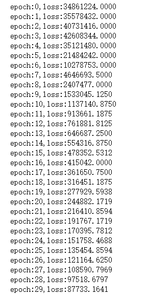
Results obtained:
4.3 torch of pytorch nn
4.3.1 torch.nn.Sequential
torch.nn. The sequential class is torch NN is a kind of Sequence container. The neural network model is built by nesting various in the container. The most important thing is that the parameters will be automatically passed down according to the sequence defined by us.
import torch
from torch.autograd import Variable
batch_n = 100#Quantity of input data for a batch
hidden_layer = 100
input_data = 1000#The characteristic of each data is 1000
output_data = 10

x = Variable(torch.randn(batch_n,input_data),requires_grad=False)
y = Variable(torch.randn(batch_n,output_data),requires_grad=False)
#Encapsulating Tensor data type variables with variables. requires_ If grad is F, it means that the gradient value of the Variable will not be retained during automatic gradient calculation.

models = torch.nn.Sequential(
    torch.nn.Linear(input_data,hidden_layer),
    torch.nn.ReLU(),
    torch.nn.Linear(hidden_layer,output_data)
)
#torch.nn.Sequential brackets are the specific structure of the neural network model we built. Linear completes the linear transformation from the hidden layer to the output layer, and then activates it with the ReLU activation function
#torch.nn. The sequential class is torch NN is a kind of Sequence container, which realizes the construction of neural network model by nesting various in the container,
#The most important thing is that the parameters will be automatically passed down according to the sequence we have defined.
4.3.2 torch.nn.Linear
torch. nn. The linear class is used to define the linear layer of the model, that is, to complete the linear transformation between the different layers mentioned above. The linear layer accepts three parameters: the number of input features, the number of output features, and whether to use offset. The default is True and torch is used nn. The linear class will automatically generate the weight parameters and offsets of the corresponding dimensions. For the generated weight parameters and offsets, our model uses a better parameter initialization method than the previous simple random method by default.
4.3.3 torch.nn.ReLU
torch.nn.ReLU belongs to the category of nonlinear activation. By default, no parameters need to be passed in during definition. Of course, in torch NN package also has many nonlinear activation function classes to choose from, such as PReLU, LeaKyReLU, Tanh, Sigmoid, Softmax, etc.
4.3.4 torch.nn.MSELoss
torch. nn. Mselos class uses the mean square error function to calculate the loss value. When defining the object of the class, you do not need to pass in any parameters, but when using an instance, you need to enter parameters with the same two dimensions.
import torch
from torch.autograd import Variable
loss_f = torch.nn.MSELoss()
x = Variable(torch.randn(100,100))
y = Variable(torch.randn(100,100))
loss = loss_f(x,y)
loss.data
#tensor(1.9529)
4.3.4 torch.nn.L1Loss
torch.nn.L1Loss class uses the average absolute error function to calculate the loss value. When defining the object of the class, you do not need to pass in any parameters, but when using the instance, you need to enter parameters with the same two dimensions for calculation.
import torch
from torch.autograd import Variable
loss_f = torch.nn.L1Loss()
x = Variable(torch.randn(100,100))
y = Variable(torch.randn(100,100))
loss = loss_f(x,y)
loss.data
#tensor(1.1356)
4.3.5 torch.nn.CrossEntropyLoss
torch. nn. The crossentropyloss class is used to calculate the cross entropy. No parameters need to be passed in when defining the object of the class, but two parameters that meet the calculation conditions of cross entropy need to be entered when using the instance.
import torch
from torch.autograd import Variable
loss_f = torch.nn.CrossEntropyLoss()
x = Variable(torch.randn(3,5))
y = Variable(torch.LongTensor(3).random_(5))#3 random numbers 0-4
loss = loss_f(x,y)
loss.data
#tensor(2.3413)
4.3. 5 neural network using loss function
import torch
from torch.autograd import Variable
import torch
from torch.autograd import Variable
loss_fn = torch.nn.MSELoss()
x = Variable(torch.randn(100,100))
y = Variable(torch.randn(100,100))
loss = loss_fn(x,y)


batch_n = 100#Quantity of input data for a batch
hidden_layer = 100
input_data = 1000#The characteristic of each data is 1000
output_data = 10

x = Variable(torch.randn(batch_n,input_data),requires_grad=False)
y = Variable(torch.randn(batch_n,output_data),requires_grad=False)
#Encapsulating Tensor data type variables with variables. requires_ If grad is F, it means that the gradient value of the Variable will not be retained during automatic gradient calculation.

models = torch.nn.Sequential(
    torch.nn.Linear(input_data,hidden_layer),
    torch.nn.ReLU(),
    torch.nn.Linear(hidden_layer,output_data)
)
#torch.nn.Sequential brackets are the specific structure of the neural network model we built. Linear completes the linear transformation from the hidden layer to the output layer, and then activates it with the ReLU activation function
#torch.nn. The sequential class is torch NN is a kind of Sequence container, which realizes the construction of neural network model by nesting various in the container,
#The most important thing is that the parameters will be automatically passed down according to the sequence we have defined.


for epoch in range(epoch_n):
    y_pred = models(x)

    loss = loss_fn(y_pred,y)
    if epoch%1000 == 0:
        print("epoch:{},loss:{:.4f}".format(epoch,loss.data))
    models.zero_grad()

    loss.backward()

    for param in models.parameters():
        param.data -= param.grad.data*lr
4.4 torch of pytorch optim
torch.optim package provides many classes that can automatically optimize parameters, such as SGD, AdaGrad, RMSProp, Adam, etc
Neural networks are implemented using automatically optimized classes:
import torch
from torch.autograd import Variable

batch_n = 100#Quantity of input data for a batch
hidden_layer = 100
input_data = 1000#The characteristic of each data is 1000
output_data = 10

x = Variable(torch.randn(batch_n,input_data),requires_grad=False)
y = Variable(torch.randn(batch_n,output_data),requires_grad=False)
#Encapsulating Tensor data type variables with variables. requires_ If grad is F, it means that the gradient value of the Variable will not be retained during automatic gradient calculation.

models = torch.nn.Sequential(
    torch.nn.Linear(input_data,hidden_layer),
    torch.nn.ReLU(),
    torch.nn.Linear(hidden_layer,output_data)
)
#torch.nn.Sequential brackets are the specific structure of the neural network model we built. Linear completes the linear transformation from the hidden layer to the output layer, and then activates it with the ReLU activation function
#torch.nn. The sequential class is torch NN is a kind of Sequence container, which realizes the construction of neural network model by nesting various in the container,
#The most important thing is that the parameters will be automatically passed down according to the sequence we have defined.

# loss_fn = torch.nn.MSELoss()
# x = Variable(torch.randn(100,100))
# y = Variable(torch.randn(100,100))
# loss = loss_fn(x,y)

epoch_n=10000
lr=1e-4
loss_fn = torch.nn.MSELoss()

optimzer = torch.optim.Adam(models.parameters(),lr=lr)
#Use torch optim. Adam class is used as the optimization function of our model parameters. What is input here is the initial value of the optimized parameters and learning rate.
#Because we need to optimize all the parameters in the model, the parameters passed are models parameters()

#The code of model training is as follows:
for epoch in range(epoch_n):
    y_pred = models(x)
    loss = loss_fn(y_pred,y)
    print("Epoch:{},Loss:{:.4f}".format(epoch,loss.data))
    optimzer.zero_grad()#Set the gradient of model parameters to 0

    loss.backward()
    optimzer.step()#The calculated gradient value is used to update the parameters of each node.
5, Building neural network to realize handwritten data set
5.1 torchvision
torchvision is a library dedicated to image processing in PyTorch. There are four categories in this package.
torchvision.datasets
torchvision.models
torchvision.transforms
torchvision.utils
5.1.1 torchvision.datasets
torchvision.datasets can download and load some datasets. For example, MNIST can use torchvision datasets. MNIST, coco, ImageNet, CIFCAR, etc. can be downloaded and loaded in this way,
Here we use torch vision Datasets load MNIST datasets:
data_train = datasets.MNIST(root="./data/",
                           transform=transform,
                           train = True,
                           download = True)
data_test = datasets.MNIST(root="./data/",
                          transform = transform,
                          train = False)
5.1.2 torchvision.models
torchvision.models provides us with trained models so that we can load them and use them directly.
torchvision. The sub modules of the models module contain the following model structures. For example:
AlexNet
VGG
ResNet
SqueezeNet
DenseNet et al
We can directly use the following code to quickly create a model with random initialization of weight:
import torchvision.models as models
resnet18 = models.resnet18()
alexnet = models.alexnet()
squeezenet = models.squeezenet1_0()
densenet = models.densenet_161()
You can also load a pre trained model by using pre trained = true:
import torchvision.models as models
resnet18 = models.resnet18(pretrained=True)
alexnet = models.alexnet(pretrained=True)
5.1.3 torch.transforms
torch. There are a large number of data transformation classes in transforms, such as:
5.1.3.1 torchvision.transforms.Resize
It is used to scale the loaded image data according to the size we need. The passed parameter can be an integer data or a sequence similar to (h,w). H stands for height and W for width. If integer data is entered, then h and W are equal to this number.
5.1.3.2 torchvision.transforms.Scale
It is used to scale the loaded image data according to the size we need. Similar to Resize.
5.1.3.3 torchvision.transforms.CenterCrop
It is used to cut the loaded picture according to the size we need with the picture center as the reference point. The parameter passed to this class can be an integer data or a sequence similar to (h,w).
5.1.3.4 torchvision.transforms.RandomCrop
It is used to randomly clip the loaded image according to the size we need. The parameter passed to this class can be an integer data or a sequence similar to (h,w).
5.1.3.5 torchvision.transforms.RandomHorizontalFlip
Used to flip the loaded picture horizontally according to random probability. We pass the custom random probability to this class. If it is not defined, the default probability is 0.5
5.1.3.6 torchvision.transforms.RandomVerticalFlip
Used to flip the loaded picture vertically according to random probability. We pass the custom random probability to this class. If it is not defined, the default probability is 0.5
5.1.3.7 torchvision.transforms.ToTensor
It is used to type convert the loaded picture data and convert the previously formed PIL picture data into a variable of Tensor data type, so that PyTorch can calculate and process it.
5.1.3.8 torchvision.transforms.ToPILImage:
It is used to convert the data of Tensor variable into PIL picture data, mainly for the convenience of picture display.
Here, use transforms to operate MNIST dataset:
#torchvision.transforms: common image transformations, such as cropping, rotation, etc;
transform=transforms.Compose(
    [transforms.ToTensor(),#Convert PILImage to tensor
     transforms.Normalize((0.5,0.5,0.5),(0.5,0.5,0.5))#Normalize [0, 1] to [- 1, 1]
     #The front (0.5, 0.5, 0.5) is the mean of R, G and B, and the back (0.5, 0.5, 0.5) is the standard deviation of the three channels
    ])
#In the above code, we can transform Compose () is regarded as a container that can combine multiple data transformations at the same time.
#The parameter passed in is a list, and the elements in the list are the transformation operations on the loaded data.
5.1.4 torch.utils
About torch vision Utils we introduce a class for loading data: torch utils. data. Dataloader and
torch. utils. data. In the dataloader class, the dataset parameter specifies the name of the dataset we load, batch_ The size parameter sets the number of pictures in each package. If shuffle is set to True, the data will be randomly disordered and packaged during loading.
data_loader_train=torch.utils.data.DataLoader(dataset=data_train,
                                       batch_size=64,#The number of pictures loaded in each batch is 1 by default. Here, it is set to 64
                                        shuffle=True,
                                        #num_workers=2#Number of subtasks required to load training data
                                       )
data_loader_test=torch.utils.data.DataLoader(dataset=data_test,
                                      batch_size=64,
                                      shuffle=True)
                                      #num_workers=2)
And torch vision utils. make_ Grid constructs a batch of pictures into grid mode pictures.
#preview
#After many attempts, it is found that the error is not caused by this sentence, but because the image format is a gray image, there is only one channel, which needs to be changed into an RGB image, so one of the lines is modified:
images,labels = next(iter(data_loader_train))
# dataiter = iter(data_loader_train) #Randomly take some data from the training data
# images, labels = dataiter.next()

img = torchvision.utils.make_grid(images)

img = img.numpy().transpose(1,2,0)
std = [0.5,0.5,0.5]
mean = [0.5,0.5,0.5]
img = img*std+mean
print([labels[i] for i in range(64)])
plt.imshow(img)
Here, iter and next obtain the picture data of a batch and its corresponding picture label, and then use torch vision utils. make_ Grid constructs a batch of pictures into a grid mode and passes through torchvision utils. make_ After grid, the picture dimension becomes channel,h,w three-dimensional. To display the picture with matplotlib, the data we want to use is an array and the dimension is (height,weight,channel), that is, the color channel is at the end. Therefore, we need to use numpy and transfer to complete the conversion of the original data type and the exchange of data dimensions.
5.2 model building and parameter optimization
Build convolution neural network model:
import math
import torch
import torch.nn as nn
class Model(nn.Module):
    def __init__(self):
        super(Model, self).__init__()

        #After constructing the convolution layer, the full connection layer and classifier are constructed
        self.conv1 = nn.Sequential(
                nn.Conv2d(3,64,kernel_size=3,stride=1,padding=1),
                nn.ReLU(),
                nn.Conv2d(64,128,kernel_size=3,stride=1,padding=1),
                nn.ReLU(),
                nn.MaxPool2d(stride=2,kernel_size=2)
                )

        self.dense = torch.nn.Sequential(
                nn.Linear(14*14*128,1024),
                nn.ReLU(),
                nn.Dropout(p=0.5),
                nn.Linear(1024,10)
            )

    def forward(self,x):
        x=self.conv1(x)
        x=x.view(-1,14*14*128)
        x=self.dense(x)
        return x
5.2.1 torch.nn.Conv2d
It is used to build the convolution layer of convolution neural network. The main parameters are:
Number of input channels, number of output channels, convolution kernel size, convolution kernel moving step and paddingde value (used for filling boundary pixels)
5.2.2 torch.nn.MaxPool2d
To realize the maximum pooling layer of convolutional neural network, the main parameters are:
The size of the pooled window, the moving step of the pooled window and the paddingde value
5.2.3 torch.nn.Dropout
It is used to prevent over fitting of convolutional neural network in the training process. The principle is to return some parameters of convolutional neural network model to zero with a certain random probability, so as to reduce the connection of two adjacent layers of neural network
5.3 parameter optimization
After building the model, we can train the model and optimize the parameters:
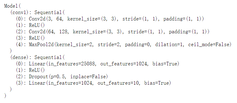
model = Model()
cost = nn.CrossEntropyLoss()
optimizer = torch.optim.Adam(model.parameters())
print(model)
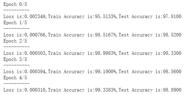
5.3. 1 model training
n_epochs = 5

for epoch in range(n_epochs):
    running_loss = 0.0
    running_correct = 0
    print("Epoch {}/{}".format(epoch,n_epochs))
    print("-"*10)
    for data in data_loader_train:
        X_train,y_train = data
        X_train,y_train = Variable(X_train),Variable(y_train)
        outputs = model(X_train)
        _,pred=torch.max(outputs.data,1)
        optimizer.zero_grad()
        loss = cost(outputs,y_train)

        loss.backward()
        optimizer.step()
        running_loss += loss.data
        running_correct += torch.sum(pred == y_train.data)
    testing_correct = 0
    for data in data_loader_test:
        X_test,y_test = data
        X_test,y_test = Variable(X_test),Variable(y_test)
        outputs = model(X_test)
        _,pred=torch.max(outputs.data,1)
        testing_correct += torch.sum(pred == y_test.data)
    print("Loss is:{:4f},Train Accuracy is:{:.4f}%,Test Accuracy is:{:.4f}".format(running_loss/len(data_train),100*running_correct/len(data_train)
                                                                                  ,100*testing_correct/len(data_test)))
5.4 model validation
In order to verify whether the trained model is really known and the results are as accurate as those displayed, the best way is to randomly select some pictures in the test set, predict with the trained model, see how much deviation there is from the real value, and visualize the results. The test code is as follows:
data_loader_test = torch.utils.data.DataLoader(dataset=data_test,
                                              batch_size = 4,
                                              shuffle = True)
X_test,y_test = next(iter(data_loader_test))
inputs = Variable(X_test)
pred = model(inputs)
_,pred = torch.max(pred,1)

print("Predict Label is:",[i for i in pred.data])
print("Real Label is:",[i for i in y_test])
img = torchvision.utils.make_grid(X_test)
img = img.numpy().transpose(1,2,0)

std = [0.5,0.5,0.5]
mean = [0.5,0.5,0.5]
img = img*std+mean
plt.imshow(img)

5.5 complete code
import torch
import torchvision
from torchvision import datasets,transforms
from torch.autograd import Variable
import numpy as np
import matplotlib.pyplot as plt

#torchvision.transforms: common image transformations, such as cropping, rotation, etc;
# transform=transforms.Compose(
#     [transforms.ToTensor(),#Convert PILImage to tensor
#      transforms.Normalize((0.5,0.5,0.5),(0.5,0.5,0.5))#Normalize [0, 1] to [- 1, 1]
#      #The front (0.5, 0.5, 0.5) is the mean of R, G and B, and the back (0.5, 0.5, 0.5) is the standard deviation of the three channels
#     ])
transform = transforms.Compose([
     transforms.ToTensor(),
     transforms.Lambda(lambda x: x.repeat(3,1,1)),
     transforms.Normalize(mean=(0.5, 0.5, 0.5), std=(0.5, 0.5, 0.5))
 ])   # Modified location

data_train = datasets.MNIST(root="./data/",
                           transform=transform,
                           train = True,
                           download = True)
data_test = datasets.MNIST(root="./data/",
                          transform = transform,
                          train = False)

data_loader_train=torch.utils.data.DataLoader(dataset=data_train,
                                       batch_size=64,#The number of pictures loaded in each batch is 1 by default. Here, it is set to 64
                                        shuffle=True,
                                        #num_workers=2#Number of subtasks required to load training data
                                       )
data_loader_test=torch.utils.data.DataLoader(dataset=data_test,
                                      batch_size=64,
                                      shuffle=True)
                                      #num_workers=2)

#preview
#After many attempts, it is found that the error is not caused by this sentence, but because the image format is a gray image, there is only one channel, which needs to be changed into an RGB image, so one of the lines is modified:
images,labels = next(iter(data_loader_train))
# dataiter = iter(data_loader_train) #Randomly take some data from the training data
# images, labels = dataiter.next()

img = torchvision.utils.make_grid(images)

img = img.numpy().transpose(1,2,0)
std = [0.5,0.5,0.5]
mean = [0.5,0.5,0.5]
img = img*std+mean
print([labels[i] for i in range(64)])
plt.imshow(img)

import math
import torch
import torch.nn as nn
class Model(nn.Module):
    def __init__(self):
        super(Model, self).__init__()

        #After constructing the convolution layer, the full connection layer and classifier are constructed
        self.conv1 = nn.Sequential(
                nn.Conv2d(3,64,kernel_size=3,stride=1,padding=1),
                nn.ReLU(),
                nn.Conv2d(64,128,kernel_size=3,stride=1,padding=1),
                nn.ReLU(),
                nn.MaxPool2d(stride=2,kernel_size=2)
                )

        self.dense = torch.nn.Sequential(
                nn.Linear(14*14*128,1024),
                nn.ReLU(),
                nn.Dropout(p=0.5),
                nn.Linear(1024,10)
            )

    def forward(self,x):
        x=self.conv1(x)
        x=x.view(-1,14*14*128)
        x=self.dense(x)
        return x

model = Model()
cost = nn.CrossEntropyLoss()
optimizer = torch.optim.Adam(model.parameters())
print(model)

n_epochs = 5

for epoch in range(n_epochs):
    running_loss = 0.0
    running_correct = 0
    print("Epoch {}/{}".format(epoch,n_epochs))
    print("-"*10)
    for data in data_loader_train:
        X_train,y_train = data
        X_train,y_train = Variable(X_train),Variable(y_train)
        outputs = model(X_train)
        _,pred=torch.max(outputs.data,1)
        optimizer.zero_grad()
        loss = cost(outputs,y_train)

        loss.backward()
        optimizer.step()
        running_loss += loss.data
        running_correct += torch.sum(pred == y_train.data)
    testing_correct = 0
    for data in data_loader_test:
        X_test,y_test = data
        X_test,y_test = Variable(X_test),Variable(y_test)
        outputs = model(X_test)
        _,pred=torch.max(outputs.data,1)
        testing_correct += torch.sum(pred == y_test.data)
    print("Loss is:{:4f},Train Accuracy is:{:.4f}%,Test Accuracy is:{:.4f}".format(running_loss/len(data_train),100*running_correct/len(data_train)
                                                                                  ,100*testing_correct/len(data_test)))

data_loader_test = torch.utils.data.DataLoader(dataset=data_test,
                                              batch_size = 4,
                                              shuffle = True)
X_test,y_test = next(iter(data_loader_test))
inputs = Variable(X_test)
pred = model(inputs)
_,pred = torch.max(pred,1)

print("Predict Label is:",[i for i in pred.data])
print("Real Label is:",[i for i in y_test])
img = torchvision.utils.make_grid(X_test)
img = img.numpy().transpose(1,2,0)

std = [0.5,0.5,0.5]
mean = [0.5,0.5,0.5]
img = img*std+mean
plt.imshow(img)
6, Conclusion
***
