In my impression, a friend asked me to write an article on how to deal with unbalanced data and sort out relevant theoretical and practical knowledge long ago, so I almost have today's article. Unbalanced samples are very common in our real world, so what problems will arise when we use these unbalanced sample data in machine learning (ML)? How to deal with these unbalanced samples? The following contents hope to help you!
00 Index
01 what is unbalanced data 02 theoretical method of processing unbalanced data 03 what package in Python can handle unbalanced samples 04 how to deal with imbalance samples in Python
01 what is unbalanced data
The unbalanced data occurs in the classification application scenario. In the classification problem, the uneven distribution between categories is the root of the imbalance. Suppose there is a binary classification problem, and the target is y, then the value range of Y is 0 and 1. When the proportion of one party (for example, y=1) is much smaller than that of the other party (y=0), it is the unbalanced sample.
So how much difference is needed to be regarded as imbalance? According to Google Developer, we can generally divide the imbalance into three levels:
- Mild: 20-40%
- Moderate: 1-20%
- Extreme: < 1%
Generally speaking, when we build the model, we can't see any problems with unbalanced samples, and often we can get high accuracy. Why? Suppose we have an extremely unbalanced sample, and the proportion of y=1 is 1%, then the model we train will tend to predict the test set as 0, so that the overall prediction accuracy of the sub model will have a good figure. If we only pay attention to this index, we may be cheated.
02 theoretical method of processing unbalanced data
Before we begin to use Python to deal with unbalanced samples, let's first understand some theoretical knowledge about dealing with unbalanced samples. The solutions of predecessors to such problems mainly include the following:
- From the perspective of data: deal with unbalanced samples by applying some under sampling or over sampling techniques. Under sampling is to sample the majority of classes and retain the total quantity of the minority to make the quantity of the two classes equal. Oversampling is to repeatedly sample the minority of classes and retain the total quantity of the majority of classes to make the quantity of the two classes equal. However, such practices also have disadvantages. Under sampling will lead to the loss of some information, which may contain some important information, and over sampling will lead to the over fitting of the classifier. Of course, it can also be the combination of the two technologies.
- From the perspective of algorithm: the solution from the perspective of algorithm is to adjust the weight of each type of training instance. For example, in a parametric classifier like SVM, grid search and cross validation can be applied to optimize C and gamma values. For nonparametric models such as decision tree, the effect can be optimized by adjusting the probability estimation on the leaf nodes. In addition, some researchers look at this kind of problems from the perspective of the combination of data and algorithms, and propose an adaptive over sampling and undersampling boost algorithm, which is a combination of the two. The novelty of this algorithm is that it adaptively oversamples a few class samples, and then undersamples most class samples to form different classifiers, These sub classifiers are combined according to their accuracy to form a powerful classifier. For more information, please refer to:
AdaOUBoost: https://dl.acm.org/doi/10.1145/1743384.1743408
03 what package in Python can handle unbalanced samples
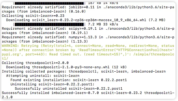
Here is a very good package called imbalanced learn. You can install it on your computer.
Official documents: https://imbalanced-learn.readthedocs.io/en/stable/index.html
pip install -U imbalanced-learn
Using the above package, we can realize the undersampling and oversampling of samples, and use pipeline to realize the combination of the two, which is very convenient. Let's use it briefly in the next section!
04 how to deal with imbalance samples in Python
For better understanding, we introduce a data set, a marketing campaign data set from the UCI machine learning repository. (data sets can be downloaded from the official website: https://archive.ics.uci.edu/ml/machine-learning-databases/00222/ Download bank additional Zip or get back to the official account to get the keyword bank.
After completing the installation of imblearn library, we can start simple operations (for other more complex operations, please refer to the official documents directly). I will demonstrate how to deal with imbalance samples with Python from four aspects: 🌈 1. Implementation of random undersampling 🌈 2. Oversampling with SMOTE 🌈 3. Combination of undersampling and oversampling (using pipeline) 🌈 4. How to obtain the best sampling rate?
🚗🚗🚗 Let's start!
# Import related libraries (mainly imblearn Library)
from collections import Counter
from sklearn.model_selection import train_test_split
from sklearn.model_selection import cross_val_score
import pandas as pd
import numpy as np
import warnings
warnings.simplefilter(action='ignore', category=FutureWarning)

from sklearn.svm import SVC
from sklearn.metrics import classification_report, roc_auc_score
from numpy import mean

# Import data
df = pd.read_csv(r'./data/bank-additional/bank-additional-full.csv', ';') # '';''  Is a separator
df.head()
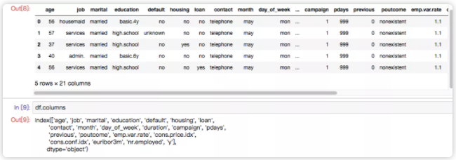
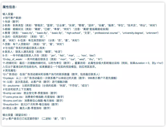
The data set is the data of a marketing campaign of Bank of Portugal. Its marketing goal is to let customers subscribe to their products, and then they form this data set through customer information obtained through telephone communication with customers and other channels. For field definitions, see the following screenshot:
We can roughly see whether the data set is an unbalanced sample:
df['y'].value_counts()/len(df)

#no     0.887346
#yes    0.112654
#Name: y, dtype: float64
It can be seen that the proportion of a few categories is 11.2%, which belongs to the sample of moderate imbalance.
# Keep only numeric variables (simple operation)
df = df.loc[:,
['age', 'duration', 'campaign', 'pdays',
       'previous', 'emp.var.rate', 'cons.price.idx',
       'cons.conf.idx', 'euribor3m', 'nr.employed','y']]
# target changed from yes/no to 0 / 1
df['y'] = df['y'].apply(lambda x: 1 if x=='yes' else 0)
df['y'].value_counts()

#0    36548
#1     4640
#Name: y, dtype: int64
🌈 1. Implementation of random undersampling
The under sampling method can also be used in the under sampling library_ sampling. RandomUnderSampler, we can use the method to be introduced, and then call it. It can be seen that there are 21942 samples in the original 0. After under sampling, it becomes the same number as 1 (i.e. 2770), realizing 50% / 50% category distribution.
# 1. Implementation of random undersampling
# Import related methods
from imblearn.under_sampling import RandomUnderSampler

# Divide dependent and independent variables
X = df.iloc[:,:-1]
y = df.iloc[:,-1]

# Divide training set and test set
X_train, X_test, y_train, y_test = train_test_split(X,y,test_size=0.40)

# Statistics on the proportion of current categories
print("Before undersampling: ", Counter(y_train))

# Call method for undersampling
undersample = RandomUnderSampler(sampling_strategy='majority')

# Obtain the sample after under sampling
X_train_under, y_train_under = undersample.fit_resample(X_train, y_train)

# Statistics on the proportion of categories after under sampling
print("After undersampling: ", Counter(y_train_under))

# Call support vector machine algorithm SVC
model=SVC()

clf = model.fit(X_train, y_train)
pred = clf.predict(X_test)
print("ROC AUC score for original data: ", roc_auc_score(y_test, pred))

clf_under = model.fit(X_train_under, y_train_under)
pred_under = clf_under.predict(X_test)
print("ROC AUC score for undersampled data: ", roc_auc_score(y_test, pred_under))

# Output:
#Before undersampling:  Counter({0: 21942, 1: 2770})
#After undersampling:  Counter({0: 2770, 1: 2770})
#ROC AUC score for original data:  0.603521152028
#ROC AUC score for undersampled data:  0.829234085179
🌈 2. Oversampling with SMOTE
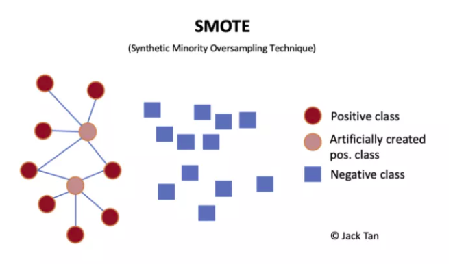
Among oversampling techniques, SMOTE is considered to be one of the most popular data sampling algorithms. It is an improved version of random oversampling algorithm. Because random oversampling only adopts the strategy of simply copying samples to amplify samples, a more direct problem will be over fitting. Therefore, the basic idea of SMOTE is to analyze a few samples and synthesize new samples to add to the data set.
The algorithm flow is as follows: (1) For each sample x in the minority class, the distance from it to all samples in the minority class sample set is calculated by taking the Euclidean distance as the standard, and its k-nearest neighbor is obtained. (2) A sampling ratio is set according to the sample imbalance ratio to determine the sampling ratio N. for each minority sample x, several samples are randomly selected from its k nearest neighbors, assuming that the selected nearest neighbor is xn. (3) For each randomly selected nearest neighbor xn, a new sample is constructed with the original sample according to the following formula.
# 2. Oversampling with SMOTE
# Import related methods
from imblearn.over_sampling import SMOTE

# Divide dependent and independent variables
X = df.iloc[:,:-1]
y = df.iloc[:,-1]

# Divide training set and test set
X_train, X_test, y_train, y_test = train_test_split(X,y,test_size=0.40)

# Statistics on the proportion of current categories
print("Before oversampling: ", Counter(y_train))

# Call method for oversampling
SMOTE = SMOTE()

# Obtain oversampled samples
X_train_SMOTE, y_train_SMOTE = SMOTE.fit_resample(X_train, y_train)

# Statistics on the proportion of categories after oversampling
print("After oversampling: ",Counter(y_train_SMOTE))

# Call support vector machine algorithm SVC
model=SVC()

clf = model.fit(X_train, y_train)
pred = clf.predict(X_test)
print("ROC AUC score for original data: ", roc_auc_score(y_test, pred))

clf_SMOTE= model.fit(X_train_SMOTE, y_train_SMOTE)
pred_SMOTE = clf_SMOTE.predict(X_test)
print("ROC AUC score for oversampling data: ", roc_auc_score(y_test, pred_SMOTE))

# Output:
#Before oversampling:  Counter({0: 21980, 1: 2732})
#After oversampling:  Counter({0: 21980, 1: 21980})
#ROC AUC score for original data:  0.602555700614
#ROC AUC score for oversampling data:  0.844305732561
🌈 3. Combination of undersampling and oversampling (using pipeline)
What if we need to use both oversampling and undersampling? In fact, it is very simple to use pipeline.
#  3. Combination of undersampling and oversampling (using pipeline)
# Import related methods
from imblearn.over_sampling import SMOTE
from imblearn.under_sampling import RandomUnderSampler
from imblearn.pipeline import Pipeline

# Divide dependent and independent variables
X = df.iloc[:,:-1]
y = df.iloc[:,-1]

#  Define pipe
model = SVC()
over = SMOTE(sampling_strategy=0.4)
under = RandomUnderSampler(sampling_strategy=0.5)
steps = [('o', over), ('u', under), ('model', model)]
pipeline = Pipeline(steps=steps)

# Evaluation effect
scores = cross_val_score(pipeline, X, y, scoring='roc_auc', cv=5, n_jobs=-1)
score = mean(scores)
print('ROC AUC score for the combined sampling method: %.3f' % score)

# Output:
#ROC AUC score for the combined sampling method: 0.937
🌈 4. How to obtain the best sampling rate?
In the above chestnuts, we all change the sampling ratio to 50:50 by default, but the sampling ratio of such chestnuts is not the optimal choice. Therefore, we introduce a concept called the optimal sampling rate, and then we find this best advantage by setting the sampling ratio and sampling grid search.
# 4. How to obtain the best sampling rate?
# Import related methods
from imblearn.over_sampling import SMOTE
from imblearn.under_sampling import RandomUnderSampler
from imblearn.pipeline import Pipeline

# Divide dependent and independent variables
X = df.iloc[:,:-1]
y = df.iloc[:,-1]

# values to evaluate
over_values = [0.3,0.4,0.5]
under_values = [0.7,0.6,0.5]
for o in over_values:
  for u in under_values:
    # define pipeline
    model = SVC()
    over = SMOTE(sampling_strategy=o)
    under = RandomUnderSampler(sampling_strategy=u)
    steps = [('over', over), ('under', under), ('model', model)]
    pipeline = Pipeline(steps=steps)
    # evaluate pipeline
    scores = cross_val_score(pipeline, X, y, scoring='roc_auc', cv=5, n_jobs=-1)
    score = mean(scores)
    print('SMOTE oversampling rate:%.1f, Random undersampling rate:%.1f , Mean ROC AUC: %.3f' % (o, u, score))


# Output:
#SMOTE oversampling rate:0.3, Random undersampling rate:0.7 , Mean ROC AUC: 0.938
#SMOTE oversampling rate:0.3, Random undersampling rate:0.6 , Mean ROC AUC: 0.936
#SMOTE oversampling rate:0.3, Random undersampling rate:0.5 , Mean ROC AUC: 0.937
#SMOTE oversampling rate:0.4, Random undersampling rate:0.7 , Mean ROC AUC: 0.938
#SMOTE oversampling rate:0.4, Random undersampling rate:0.6 , Mean ROC AUC: 0.937
#SMOTE oversampling rate:0.4, Random undersampling rate:0.5 , Mean ROC AUC: 0.938
#SMOTE oversampling rate:0.5, Random undersampling rate:0.7 , Mean ROC AUC: 0.939
#SMOTE oversampling rate:0.5, Random undersampling rate:0.6 , Mean ROC AUC: 0.938
#SMOTE oversampling rate:0.5, Random undersampling rate:0.5 , Mean ROC AUC: 0.938
From the result log, the optimal sampling rate is oversampling 0.5 and undersampling 0.7.
Finally, I want to tell you that there is no absolute routine, only the appropriate routine, whether under sampling or over sampling, only the appropriate is the most important. In addition, under sampling will indeed "save money" than over sampling (it can be felt intuitively from the training time).
References
[1] SMOTE algorithm https://www.jianshu.com/p/13fc0f7f5565 [2] How to deal with imbalanced data in Python