1, Write in front
This article introduces an improved version of RNN - LSTM on the basis of my other blog post "understanding RNN in one article"
2, LSTM
In the practical application of RNN, we find that when the number of time steps is large or the time steps are small, the gradient of cyclic neural network is prone to attenuation or explosion. Although clipping gradient can deal with gradient explosion, it can not solve the problem of gradient attenuation. Usually for this reason, it is difficult to capture the dependence of time step distance in time series in practice. In order to solve this problem, scholars have proposed GRU model and LSTM model. LSTM model is more complex than GRU model and has more gating mechanisms, so the effect is generally better.
2.1 input gate, forgetting gate and output gate
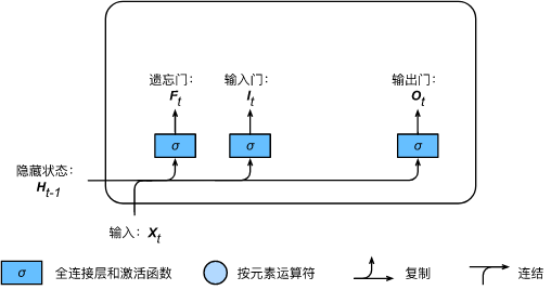
LSTM introduces three gates, namely input gate, forget gate and output gate, as well as memory cells with the same shape as the hidden state (some literatures regard memory cells as a special hidden state), so as to record additional information.
2.2 input gate, forgetting gate and output gate
Like the reset door and update door in the door control cycle unit, as shown in the figure below, the input of the door of long-term and short-term memory is the current time step input
X
t
\boldsymbol{X}t
Xt and previous time step hidden state
H
t
−
1
\boldsymbol{H}{t-1}
Ht − 1, the output is calculated by the full connection layer whose activation function is sigmoid function. In this way, the value range of the three gate elements is
[
0
,
1
]
[0,1]
[0,1].
Specifically, assume that the number of hidden units is
h
h
h. Given time step
t
t
Small batch input of t
X
t
∈
R
n
×
d
\boldsymbol{X}_t \in \mathbb{R}^{n \times d}
Xt∈Rn × d (number of samples is)
n
n
n. The number of entries is
d
d
d) And previous time step hidden status
H
t
−
1
∈
R
n
×
h
\boldsymbol{H}_{t-1} \in \mathbb{R}^{n \times h}
Ht−1∈Rn × h. Time step
t
t
t input gate
I
t
∈
R
n
×
h
\boldsymbol{I}_t \in \mathbb{R}^{n \times h}
It∈Rn × h. Forgetting gate
F
t
∈
R
n
×
h
\boldsymbol{F}_t \in \mathbb{R}^{n \times h}
Ft∈Rn × h and output gate
O
t
∈
R
n
×
h
\boldsymbol{O}_t \in \mathbb{R}^{n \times h}
Ot∈Rn × h is calculated as follows:
I t = σ ( X t W x i + H t − 1 W h i + b i ) , F t = σ ( X t W x f + H t − 1 W h f + b f ) , O t = σ ( X t W x o + H t − 1 W h o + b o ) , \begin{aligned} \boldsymbol{I}_t &= \sigma(\boldsymbol{X}_t \boldsymbol{W}_{xi} + \boldsymbol{H}_{t-1} \boldsymbol{W}_{hi} + \boldsymbol{b}i),\ \boldsymbol{F}_t &= \sigma(\boldsymbol{X}_t \boldsymbol{W}_{xf} + \boldsymbol{H}_{t-1} \boldsymbol{W}_{hf} + \boldsymbol{b}_f),\ \boldsymbol{O}_t &= \sigma(\boldsymbol{X}t \boldsymbol{W}_{xo} + \boldsymbol{H}_{t-1} \boldsymbol{W}_{ho} + \boldsymbol{b}_o), \end{aligned} It=σ(XtWxi+Ht−1Whi+bi), Ft=σ(XtWxf+Ht−1Whf+bf), Ot=σ(XtWxo+Ht−1Who+bo),
Among them W x i , W x f , W x o ∈ R d × h \boldsymbol{W}{xi}, \boldsymbol{W}{xf}, \boldsymbol{W}{xo} \in \mathbb{R}^{d \times h} Wxi,Wxf,Wxo∈Rd × h and W h i , W h f , W h o ∈ R h × h \boldsymbol{W}{hi}, \boldsymbol{W}{hf}, \boldsymbol{W}{ho} \in \mathbb{R}^{h \times h} Whi,Whf,Who∈Rh × h is the weight parameter, b i , b f , b o ∈ R 1 × h \boldsymbol{b}_i, \boldsymbol{b}_f, \boldsymbol{b}_o \in \mathbb{R}^{1 \times h} bi,bf,bo∈R1 × h is the deviation parameter.
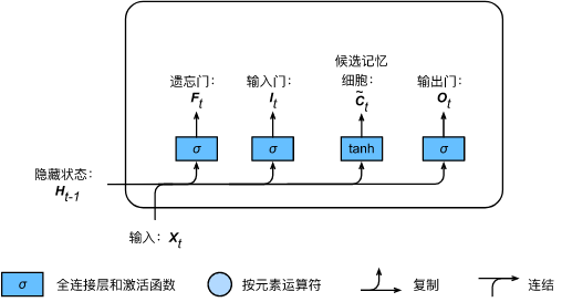
2.3 candidate memory cells
We can use the element value field in
[
0
,
1
]
[0, 1]
The input gate, forgetting gate and output gate of [0,1] control the flow of information in the hidden state, which is also generally through the use of multiplication by element (symbol
⊙
\odot
⊙) to achieve. Current time step memory cell
C
t
∈
R
n
×
h
\boldsymbol{C}_t \in \mathbb{R}^{n \times h}
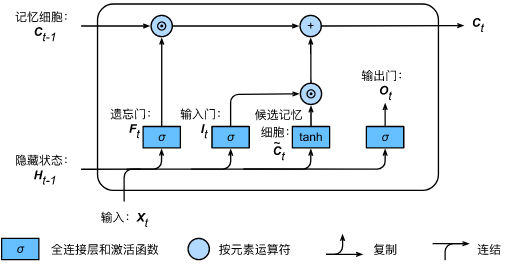
Ct∈Rn × The calculation of h combines the information of memory cells in the previous time step and candidate memory cells in the current time step, and controls the flow of information through forgetting gate and input gate:
C
t
=
F
t
⊙
C
t
−
1
+
I
t
⊙
C
~
t
.
\boldsymbol{C}_t = \boldsymbol{F}_t \odot \boldsymbol{C}_{t-1} + \boldsymbol{I}_t \odot \tilde{\boldsymbol{C}}_t.
Ct=Ft⊙Ct−1+It⊙C~t.
As shown in the figure above, the forgetting gate controls the memory cells in the previous time step
C
t
−
1
\boldsymbol{C}_{t-1}
Whether the information in Ct − 1 is transferred to the current time step, and the input gate controls the input of the current time step
X
t
\boldsymbol{X}_t
Xt) through candidate memory cells
C
~
t
\tilde{\boldsymbol{C}}_t
How C~t# flows into the memory cells of the current time step. If the forgetting gate is always close to 1 and the input gate is always close to 0, the past memory cells will always be saved through time and transferred to the current time step. This design can deal with the gradient attenuation problem in cyclic neural network and better capture the dependence of large time step distance in time series.
2.4 hidden status
After having memory cells, we can also control from memory cells to hidden state through output gate H t ∈ R n × h \boldsymbol{H}_t \in \mathbb{R}^{n \times h} Ht∈Rn × h. flow of information:
H t = O t ⊙ tanh ( C t ) . \boldsymbol{H}_t = \boldsymbol{O}_t \odot \text{tanh}(\boldsymbol{C}_t). Ht=Ot⊙tanh(Ct).
The tanh function here ensures that the value of the hidden state element is between - 1 and 1. It should be noted that when the output gate is approximately 1, the memory cell information will be transferred to the hidden state for use by the output layer; When the output gate is approximately 0, the memory cell information is only retained by itself. The figure below shows the calculation of hidden state in long-term and short-term memory.
last,
H
t
\boldsymbol{H}_t
The information in Ht ¢ is multiplied by the output matrix and the output gate offset to obtain the output result.
The above is the general process of information flow in LSTM. However, in the process of practical application, when encountering text information, the information contained in the current word is related not only to the words in the previous time steps, but also to the words after the word. Therefore, it is necessary to consider the sequence information before and after the word at the same time. Therefore, the bidirectional cyclic neural network came into being.
2.4 bidirectional cyclic neural network
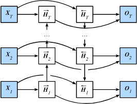
The previously introduced cyclic neural network models assume that the current time step is determined by the sequence of earlier time steps, so they all transfer information from front to back through the hidden state. Sometimes, the current time step may also be determined by the later time step. For example, when we write a sentence, we may modify the words in front of the sentence according to the words behind the sentence. Bidirectional recurrent neural network can deal with this kind of information more flexibly by adding a hidden layer that transmits information from back to front. The following figure illustrates the structure of a bidirectional cyclic neural network.
Let's introduce our definition. Given time step
t
t
Small batch input of t
X
t
∈
R
n
×
d
\boldsymbol{X}_t \in \mathbb{R}^{n \times d}
Xt∈Rn × d (number of samples is)
n
n
n. The number of entries is
d
d
d) And hidden layer activation functions are
ϕ
\phi
ϕ. In the architecture of bidirectional recurrent neural network, the forward hidden state of the time step is set as
H
→
t
∈
R
n
×
h
\overrightarrow{\boldsymbol{H}}_t \in \mathbb{R}^{n \times h}
H
t∈Rn × h (the number of forward hidden units is
h
h
h) , the reverse hide status is
H
←
t
∈
R
n
×
h
\overleftarrow{\boldsymbol{H}}_t \in \mathbb{R}^{n \times h}
H
t∈Rn × h (number of reverse hidden units is)
h
h
h). We can calculate the forward hidden state and reverse hidden state respectively:
H
→
t
=
ϕ
(
X
t
W
x
h
(
f
)
+
H
→
t
−
1
W
h
h
(
f
)
+
b
h
(
f
)
)
,
H
←
t
=
ϕ
(
X
t
W
x
h
(
b
)
+
H
←
t
+
1
W
h
h
(
b
)
+
b
h
(
b
)
)
,
\begin{aligned} \overrightarrow{\boldsymbol{H}}t &= \phi(\boldsymbol{X}t \boldsymbol{W}{xh}^{(f)} + \overrightarrow{\boldsymbol{H}}{t-1} \boldsymbol{W}_{hh}^{(f)} + \boldsymbol{b}h^{(f)}),\ \overleftarrow{\boldsymbol{H}}t &= \phi(\boldsymbol{X}t \boldsymbol{W}{xh}^{(b)} + \overleftarrow{\boldsymbol{H}}{t+1} \boldsymbol{W}{hh}^{(b)} + \boldsymbol{b}_h^{(b)}), \end{aligned}
H
t=ϕ(XtWxh(f)+H
t−1Whh(f)+bh(f)), H
t=ϕ(XtWxh(b)+H
t+1Whh(b)+bh(b)),
Where weight W x h ( f ) ∈ R d × h \boldsymbol{W}{xh}^{(f)} \in \mathbb{R}^{d \times h} Wxh(f)∈Rd×h, W h h ( f ) ∈ R h × h \boldsymbol{W}{hh}^{(f)} \in \mathbb{R}^{h \times h} Whh(f)∈Rh×h, W x h ( b ) ∈ R d × h \boldsymbol{W}{xh}^{(b)} \in \mathbb{R}^{d \times h} Wxh(b)∈Rd×h, W h h ( b ) ∈ R h × h \boldsymbol{W}{hh}^{(b)} \in \mathbb{R}^{h \times h} Whh(b)∈Rh × h and deviation b h ( f ) ∈ R 1 × h \boldsymbol{b}_h^{(f)} \in \mathbb{R}^{1 \times h} bh(f)∈R1×h, b h ( b ) ∈ R 1 × h \boldsymbol{b}_h^{(b)} \in \mathbb{R}^{1 \times h} bh(b)∈R1 × h are all model parameters.
Then we link the hidden states in both directions H → t \overrightarrow{\boldsymbol{H}}_t H t , and H ← t \overleftarrow{\boldsymbol{H}}_t H t , to get the hidden state H t ∈ R n × 2 h \boldsymbol{H}_t \in \mathbb{R}^{n \times 2h} Ht∈Rn × 2h and input it to the output layer. Output layer calculation output O t ∈ R n × q \boldsymbol{O}_t \in \mathbb{R}^{n \times q} Ot∈Rn × q (number of outputs is) q q q):
O t = H t W h q + b q , \boldsymbol{O}_t = \boldsymbol{H}t \boldsymbol{W}{hq} + \boldsymbol{b}_q, Ot=HtWhq+bq,
Where weight W h q ∈ R 2 h × q \boldsymbol{W}_{hq} \in \mathbb{R}^{2h \times q} Whq∈R2h × q and deviation b q ∈ R 1 × q \boldsymbol{b}_q \in \mathbb{R}^{1 \times q} bq∈R1 × q is the model parameter of the output layer. The number of hidden cells in different directions can also be different.
3, Implementing BiLSTM emotion analysis with pytorch
Next, with the help of pytorch framework, a text classification model is established to classify the text emotion and apply it to the subsequent recommendation system.
3.1 data reading and preprocessing
First, we read the data set and put a positive label on the comments corresponding to the score of 4-5; Comments with a score below 4 are labeled negative. Then we divide the training test set in a ratio of 1:1.
import pandas as pd
from d2lzh_pytorch import evaluate_accuracy
import collections
import os
import random
import tarfile
import torch
from torch import nn
import torchtext.vocab as Vocab
import torch.utils.data as Data
import time
import sys
sys.path.append("..")
data=pd.read_csv('data_children_sorted2.csv')
data=data[['rating','review_text']]#Only score and comment text
li=data['rating']
a=[]
for i in li:
    if int(i)>3:
        a.append('pos')
    else:
        a.append('neg')
data['target']=a
data=data.dropna()
sum=0
for i in data['review_text']:
    sum+=len(i)
print('mean:',sum//len(data))
device = torch.device('cuda' if torch.cuda.is_available() else 'cpu')
data_=[]
for review,label in zip(data['review_text'],data['target']):
    data_.append([review, 1 if label == 'pos' else 0])
mid=len(data_)//2
train=data_[:mid]
test=data_[mid:]
We need to segment each comment to get a comment with a good word. Get defined here_ tokenized_ The IMDB function uses the simplest method: word segmentation based on spaces.
def get_tokenized_imdb(data):#participle
    """
    data: list of [string, label]
    """
    def tokenizer(text):
        return [tok.lower() for tok in text.split(' ')]
    return [tokenizer(review) for review, _ in data]
Now we can create a dictionary based on the training data set of divided words. Here we filter out words that appear less than 5 times.
def get_vocab_imdb(data):
    tokenized_data = get_tokenized_imdb(data)
    counter = collections.Counter([tk for st in tokenized_data for tk in st])
    return Vocab.Vocab(counter, min_freq=5)
#Count word frequency and filter out words with word frequency less than 5
vocab = get_vocab_imdb(data_)
Because the length of each comment is inconsistent, it cannot be directly combined into a small batch. We define preprocess_ The IMDB function divides each comment into words, converts it into a word index through a dictionary, and then fixes the length of each comment to 500 by truncating or complementing 0.
def preprocess_imdb(data,vocab):#The shorter text is lengthened and the longer text is cropped to obtain a unified long sequence
    max_l=500
    def pad(x):
        return x[:max_l] if len(x)>max_l else x+[0]*(max_l-len(x))
    tokenized_data=get_tokenized_imdb(data)
    features=torch.tensor([pad([vocab.stoi[word] for word in words]) for words in tokenized_data])
    labels = torch.tensor([score for _,score in data])
    return features,labels
3.2 creating data iterators
Now let's create a data iterator. Each iteration will return a small batch of data.
batch_size = 64
train_set = Data.TensorDataset(*preprocess_imdb(train_data, vocab))
test_set = Data.TensorDataset(*preprocess_imdb(test_data, vocab))
train_iter = Data.DataLoader(train_set, batch_size, shuffle=True)
test_iter = Data.DataLoader(test_set, batch_size)
3.3 model using cyclic neural network
In this model, each word first gets the feature vector through the Embedding layer. Then, we use bidirectional recurrent neural network to further encode the characteristic sequence to obtain the sequence information. Finally, we transform the encoded sequence information into output through the full connection layer. Specifically, we can link the hidden states of bidirectional long-term and short-term memory in the initial time step and the final time step as the representation of the feature sequence to the output layer classification. In the BiRNN class implemented below, the Embedding instance is the Embedding layer, the LSTM instance is the hidden layer of sequence coding, and the Linear instance is the output layer that generates classification results.
class BiRNN(nn.Module):
    def __init__(self, vocab, embed_size, num_hiddens, num_layers):
        super(BiRNN, self).__init__()
        self.embedding = nn.Embedding(len(vocab), embed_size)
        # When bidirectional is set to True, a bidirectional recurrent neural network is obtained
        self.encoder = nn.LSTM(input_size=embed_size,
                                hidden_size=num_hiddens,
                                num_layers=num_layers,
                                bidirectional=True)
        # The hidden states of the initial time step and the final time step are input as the full connection layer
        self.decoder = nn.Linear(4*num_hiddens, 2)

    def forward(self, inputs):
        # The shape of inputs is (batch size, number of words). Because LSTM needs to take the sequence length (seq_len) as the first dimension, the input will be transposed
        # Then extract word features, and the output shape is (number of words, batch size, word vector dimension)
        embeddings = self.embedding(inputs.permute(1, 0))
        # rnn.LSTM only passes in the input embeddings, so it only returns the hidden state of the last hidden layer in each time step.
        # outputs shape is (number of words, batch size, 2 * number of hidden units)
        outputs, _ = self.encoder(embeddings) # output, (h, c)
        # Connect the hidden state of the initial time step and the final time step as the full connection layer input. Its shape is
        # (batch size, 4 * number of hidden units).
        encoding = torch.cat((outputs[0], outputs[-1]), -1)
        outs = self.deco
Create a bidirectional recurrent neural network with two hidden layers.
embed_size, num_hiddens, num_layers = 100, 100, 2
net = BiRNN(vocab, embed_size, num_hiddens, num_layers)
3.4 loading pre trained word vector
Due to the large data of emotion analysis, in order to reduce the training time and improve the quality of word vectors, and deal with over fitting, we will directly use the word vectors pre trained on a larger corpus as the feature vectors of each word. Here, we load a 100 dimensional GloVe word vector for each word in the dictionary vocab.
DATA_ROOT='C:/Users/wuyang/Datasets'
glove_vocab=Vocab.GloVe(name='6B',dim=100,cache=os.path.join(DATA_ROOT, "glove"))#Load pre training word vector
Then, we will use these word vectors as the feature vectors of each word in the comment. Note that the dimension of the pre training word vector needs to be embedded with the output size of the embedded layer in the created model_ Consistent size. In addition, we will not update these word vectors in training.
# This function has been saved in d2lzh_torch package for later use
def load_pretrained_embedding(words, pretrained_vocab):
    """From pre training vocab Extracted from words Corresponding word vector"""
    embed = torch.zeros(len(words), pretrained_vocab.vectors[0].shape[0]) # Initialize to 0
    oov_count = 0 # out of vocabulary
    for i, word in enumerate(words):
        try:
            idx = pretrained_vocab.stoi[word]
            embed[i, :] = pretrained_vocab.vectors[idx]
        except KeyError:
            oov_count += 1
    if oov_count > 0:
        print("There are %d oov words." % oov_count)
    return embed

net.embedding.weight.data.copy_(
    load_pretrained_embedding(vocab.itos, glove_vocab))
net.embedding.weight.requires_grad = False # Load the pre trained directly, so you don't need to update it
Then you can start training the model.
lr, num_epochs = 0.01, 5
# The embedding parameters that do not calculate the gradient should be filtered out. Because the pre training word vector is used for loading, the embedding layer does not update the parameters and the gradient does not exist
optimizer = torch.optim.Adam(filter(lambda p: p.requires_grad, net.parameters()), lr=lr)
loss = nn.CrossEntropyLoss()
def train(train_iter, test_iter, net, loss, optimizer, device, num_epochs):
    net = net.to(device)
    print("training on ", device)
    batch_count = 0
    for epoch in range(num_epochs):
        train_l_sum, train_acc_sum, n, start = 0.0, 0.0, 0, time.time()
        for X, y in train_iter:
            X = X.to(device)
            y = y.to(device)
            y_hat = net(X)
            l = loss(y_hat, y)
            optimizer.zero_grad()
            l.backward()
            optimizer.step()
            train_l_sum += l.cpu().item()
            train_acc_sum += (y_hat.argmax(dim=1) == y).sum().cpu().item()
            n += y.shape[0]
            batch_count += 1
        test_acc = evaluate_accuracy(test_iter, net)
        print('epoch %d, loss %.4f, train acc %.3f, test acc %.3f, time %.1f sec'
              % (epoch + 1, train_l_sum / batch_count, train_acc_sum / n, test_acc, time.time() - start))
train(train_iter, test_iter, net, loss, optimizer, device, num_epochs)
Training results:
training on  cuda
epoch 1, loss 0.5759, train acc 0.666, test acc 0.832, time 250.8 sec
epoch 2, loss 0.1785, train acc 0.842, test acc 0.852, time 253.3 sec
epoch 3, loss 0.1042, train acc 0.866, test acc 0.856, time 253.7 sec
epoch 4, loss 0.0682, train acc 0.888, test acc 0.868, time 254.2 sec
epoch 5, loss 0.0483, train acc 0.901, test acc 0.862, time 251.4 sec
Overall, the effect is very good.