The content of this article comes from learning MIT open course: univariate calculus - the second basic theorem of calculus - Netease open course

1, In reverse, FTC1

FTC1: if F'(x) = f(x),

On the contrary:

Use f to understand F and f '

The information of F 'can be derived from the information of F

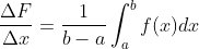
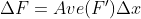
1. Compare FTC1 and mean value theorem

...... (here)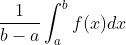Is the average of f)

Inequality Description:

...... (here f 'and F are the same thing, there is no difference)

So why is this average not the average of F, but the average of F '?

Because this formula is to find the accumulation of f(x) from a to b

The teacher gave an example

a=0, b=n

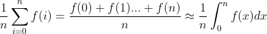
The left side of the equation is the discrete mean, while the right side is the continuous mean. (personal feeling is not a good example)

Personally, I think that the integral is actually the sum of the area of the figure surrounded by f(x) and X axis. It can be thought of as a figure composed of countless thin rectangles. Therefore, when dividing the figure into n equal parts, the function values of each part are added to find the average( 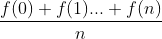, the average of the height of the rectangle) and then multiplied by the coverage of the x-axis (e.g b-a, the length of the bottom edge of the rectangle), you can get an approximate area value, that is And obviously when , so

from sympy import *
import numpy as np 

import matplotlib.pyplot as plt 

fig = plt.figure()
ax = fig.add_subplot(1, 1, 1)
ax.spines['left'].set_position('zero')
ax.spines['bottom'].set_position('zero')
ax.spines['right'].set_color('none')
ax.spines['top'].set_color('none')
ax.xaxis.set_ticks_position('bottom')
ax.yaxis.set_ticks_position('left')
ax.set_aspect(1 ) 

def DrawXY(xFrom,xTo,steps,expr,color,label,plt):
    yarr = []
    xarr = np.linspace(xFrom ,xTo, steps) 
    for xval in xarr:
        yval = expr.subs(x,xval)
        yarr.append(yval)
    y_nparr = np.array(yarr) 
    plt.plot(xarr, y_nparr, c=color, label=label)    

def DrawRects(xFrom,xTo,steps,expr,color,plt, label=''):
    width = (xTo - xFrom)/steps
    xarrRect = []
    yarrRect = []
    area = 0
    xprev = xFrom
    yvalAll =  0
    for step in range(steps):
        yval = expr.subs(x,xprev + width)
        xarrRect.append(xprev)
        xarrRect.append(xprev)
        xarrRect.append(xprev + width)
        xarrRect.append(xprev + width)
        xarrRect.append(xprev)
        yarrRect.append(0)
        yarrRect.append(yval)
        yarrRect.append(yval)
        yarrRect.append(0)
        yarrRect.append(0)
        area += width * yval
        plt.plot(xarrRect, yarrRect, c=color)    
        xprev= xprev + width
        yvalAll += yval
    print('============================')    
    if len(label)!=0:
        print(label)    
    print('============================')
    print('width = ', width)
    print('ave = ', yvalAll / steps)
    print('area = ',area)
    areaFinal = (integrate(expr, (x,xFrom,xTo)))
    print ('area final = ',areaFinal)
    print ('ave final = ', areaFinal / (xTo - xFrom))

def TangentLine(exprY,x0Val,xVal):
    diffExpr = diff(exprY)
    x1,y1,xo,yo = symbols('x1 y1 xo yo')
    expr = (y1-yo)/(x1-xo) - diffExpr.subs(x,x0Val)
    eq = expr.subs(xo,x0Val).subs(x1,xVal).subs(yo,exprY.subs(x,x0Val))
    eq1 = Eq(eq,0)
    solveY = solve(eq1)
    return xVal,solveY

def DrawTangentLine(exprY, x0Val,xVal1, xVal2, clr, txt):
    x1,y1 = TangentLine(exprY, x0Val, xVal1)
    x2,y2 = TangentLine(exprY, x0Val, xVal2)
    plt.plot([x1,x2],[y1,y2], color = clr, label=txt)
    
def Newton(expr, x0):
    ret = x0 - expr.subs(x, x0)/ expr.diff().subs(x,x0)
    return ret

   
x = symbols('x')
expr = x


DrawXY(0,10,10,expr,'blue','',plt)
DrawRects(0,10,10,expr,'green',plt)


#plt.legend(loc='lower right')
plt.show()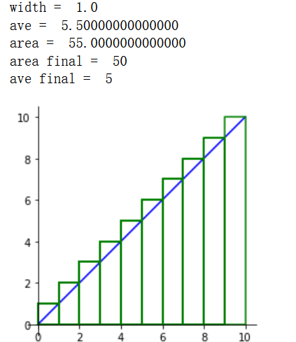

​

 

FTC1

Mean value theorem (MVT)

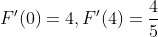
2, Exam Practice

1,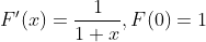

The mean value theorem implies that A < f (4) < B, find A, B

(according to the mean value theorem, here 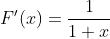Greater than 0, the range of x (0,4), so F is increasing)

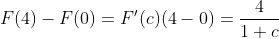(according to the mean value theorem, 0 < C < 4)

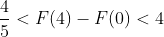
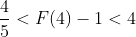
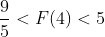
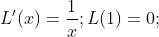
FTC1: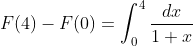

I don't quite understand why to calculate this here. It may be necessary to calculate inequalities like this in practical application

Obviously, according to the substitution method

u = 1+x, du = dx

Geometry:

 

x = symbols('x')
expr = 1/(1+x)

DrawXY(0,4,100,expr,'green','f(x) = 1/(1+x)',plt)
DrawRects(0,4,50,expr,'green',plt, 'f(x) = 1/(1+x)')

expr = 1*x**0
DrawXY(0,4,100,expr,'blue','f(x) = 1',plt)
DrawRects(0,4,1,expr,'blue',plt,'f(x) = 1')

expr = 1/(5*x**0)
DrawXY(0,4,100,expr,'red','f(x) = 1/5',plt)
DrawRects(0,4,1,expr,'red',plt,'f(x) = 1/5')

plt.legend(loc='lower right')
plt.show()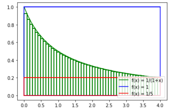

Upper and Lower riemann sum

It is easy to see the size relationship of this area from the graph. This large blue rectangle is actually the maximum value of the function during integral summation, and only one rectangle is divided (also known as Upper RS). This small red rectangle is the minimum value of the function during integral summation, and only one rectangle is divided (also known as Lower RS)

The teacher said at this time that based on the above, we can basically avoid using the mean value theorem, because there is such a better method that we can get any boundary obtained by the mean value theorem with simple integration.

3, Second fundamental theorem of calculus (FTC2)

1. Definition: if function f is continuous, and At the same time, when a and X are calculated as constants), G'(x) = f(x)

2. Purpose: G(x) can be used to solve the following differential equations

(necessary conditions)

The teacher said that the differential equation is not always solvable, but with the above premise, the differential equation always has a solution

3. Examples

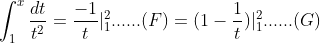
(1),

The teacher's solution here is:

In FTC2, due to

Later, the teacher's supplement to this example:

4. Prove

​

 

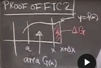
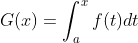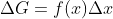
From the above figure , this G(x) is the area enclosed by the curve f(x) in the interval (0,a) and the X axis at the position indicated by the arrow. Consider In the above figure, dG is the red filled part Very small, this part of the figure is similar to a rectangle, and the height of the rectangle is y = f(x) indicated by the arrow, and its area is equal to the height of the bottom x, that is , ,

(F is continuous because f needs to have a valid value)

, there are

4, Proof of the first fundamental theorem of calculus (FTC1)

F '= f (F is continuous)

have

According to ftc2, G '(x) = f (x), F' = f

(c is constant)

from , substitute b and a respectively

5, Focus of FTC2

By FTC2, 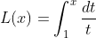(subscript 1 because L(1) = 0)

FTC2 has many new functions for a long time:

such as The area enclosed by the bell function on the (0,x) and X axes cannot be represented by any other function. Because it has completely exceeded the scope of algebra, it is called transcendental function.

Try it here

x = symbols('x')
expr = np.e**(-x**2)

DrawXY(0,2,100,expr,'green','f(x) =np.e**(-x**2)',plt)
DrawRects(0,2,50,expr,'green',plt, 'f(x) = np.e**(-x**2)')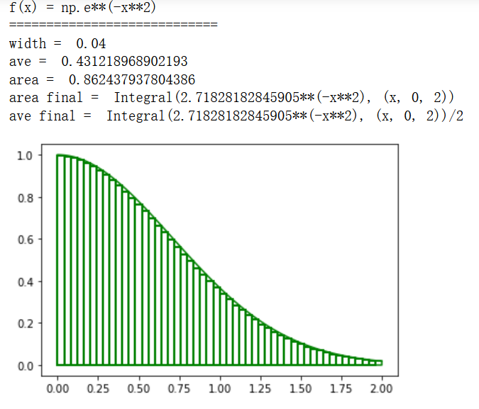

​

 

From the above results, we can see that the value of this area can not be calculated by algebraic method, but can only be approximately calculated by more divided rectangles

In addition, the teacher mentioned , this is a transcendental number, which cannot be expressed in algebra. In addition, e is also a transcendental number.