Taking the simple pendulum model as an example, the gray box identification is carried out.

1. Simple pendulum model

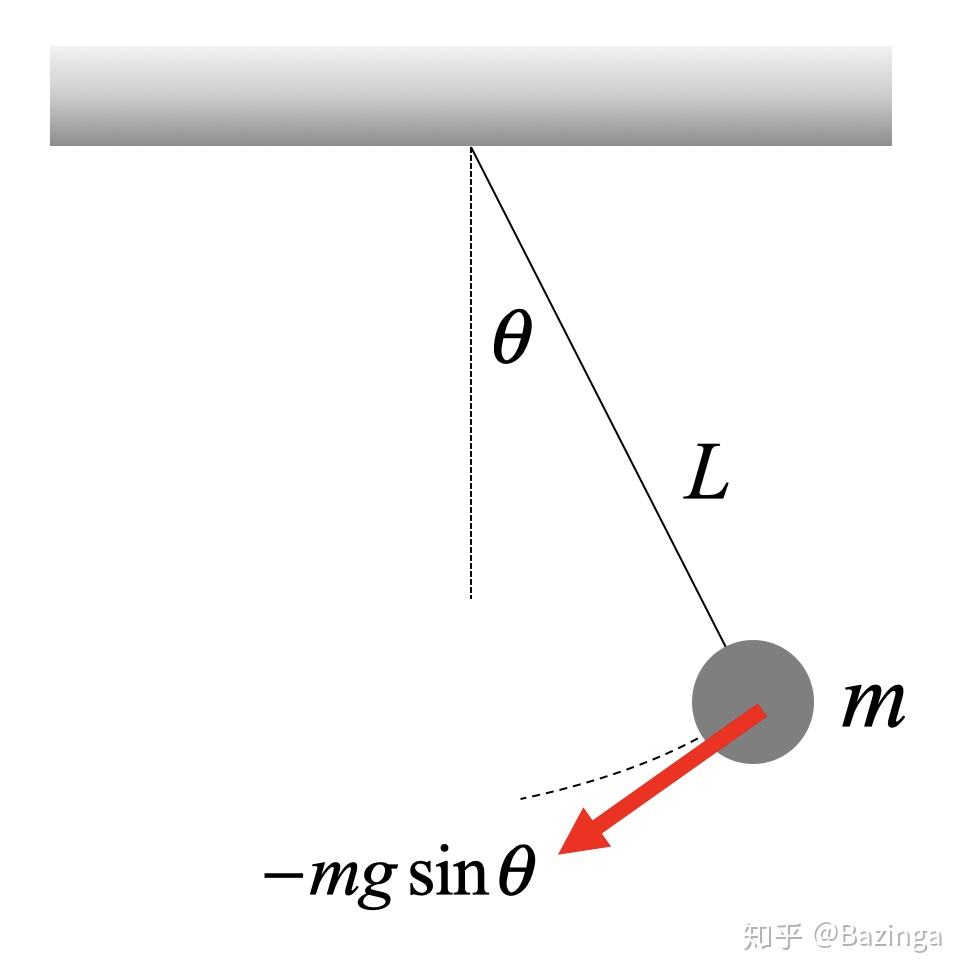
Figure 1 tangent force diagram of simple pendulum

The tangent force diagram of a simple pendulum is shown in Figure 1, and the picture comes from the network.

The equation of motion in tangent direction can be simply written out

WhereRepresents the length of the pendulum,Represents the mass of the pendulum,Is the acceleration of gravity,It represents the included angle between the simple pendulum and the vertical axis of the fixed point. It is assumed that there is a friction resistance that hinders the movement, the resistance is directly proportional to the speed, and the friction coefficient is.

Fetch state variable，And consider the moment of the simple pendulum, the moment is regarded as the control input of the simple pendulum system and written into the state space equation in the following form

2. Usage of MATLAB identification function

Here, we mainly refer to the official help document of matlab to briefly explain the usage of nlgreyest function.

Function form

sys= nlgreyest(data,init_sys)
sys= nlgreyest(data,init_sys,options)

describe

sys= nlgreyest(data,init_sys) use time domain data (data) to estimate the parameters of nonlinear system (init_sys); If there are additional estimation requirements, you can fill in the options option.

Among them, the nonlinear system init_ The model of sys needs to be established by idnlgrey function

Function form

sys = idnlgrey(FileName,Order,Parameters)
sys = idnlgrey(FileName,Order,Parameters,InitialStates)
sys = idnlgrey(FileName,Order,Parameters,InitialStates,Ts)
sys = idnlgrey(FileName,Order,Parameters,InitialStates,Ts,Name,Value)

describe

idnlgrey function creates a gray box model according to the described structure, number of inputs and outputs, order, parameters, initial state, etc.

The input and output data of the system needs to be established by iddata function

Function form

data = iddata(y,u,Ts)

describe

Iddata creates an iddata data object according to the time domain output signal y, the time domain input signal u and the sampling time Ts.

Let's try it directly, which is more intuitive.

3. Identification process of grey box model

3.1 system simulation data

Call the model set in simulink for simulation experiment.

%%
%System simulation and parameter setting
% Pendulum model
% Gravity
g = 9.81; % [m/s^2]
% Pendulum mass
m = 1; % [kg]
% Pendulum length
l = 0.5; % [m]
zn=0.1;%Damping coefficient
% Measurement noise covariance
R = 1e-2;
% Sampling time
Ts2 = 0.01; % [s]

out=sim('pendulum_line');

3.2 # define the model function of simple pendulum

The output equation and state equation are defined according to the system model, and the system model parameters are replaced by a1, a2 and a3

function [dx,y]=pendulum(t,x,u,a1,a2,a3,varargin)
y=x(1);%Output equation
dx=[x(2);
    a1*sin(x(1))+a2*x(2)+a3*u];%state equation 
end

3.3 # define the gray box model

%utilize idnlgrey Function to define the grey box model of the system
FileName='pendulum';
Order=[1 1 2];%It represents input order 1, output order 1 and state order 2 respectively
Parameters=[-10;-1;1/m*l^2];%Initial parameters
InitialStates=[pi/2;0];%Initial state
Ts=0;%Sampling time, 0 corresponds to continuous system
Sys=idnlgrey(FileName,Order,Parameters,InitialStates,Ts,...
    'Name','S_Model',...
    'InputName',{'T'},...
    'OutputName',{'theta'});
Sys=setpar(Sys,'Name',{'a1';'a2';'a3'});%Set the parameter name of the model
Sys.Parameters(3).Fixed = true;%hypothesis m and l Known, so this parameter is fixed

3.4 system parameter identification

%%
%System parameter identification

%1.Read data
data=[out.simin.signals.values,out.simout.signals.values];
Z=data(:,2);%system output 
N=length(Z);%Data length
u=data(:,1);%System input
data2=iddata(Z,u,Ts2);

%2.Grey box model identification
Sys=nlgreyest(data2,Sys,nlgreyestOptions('Display','on'));
figure;
compare(data2,Sys);%Comparison of identification results

3.5 identification results

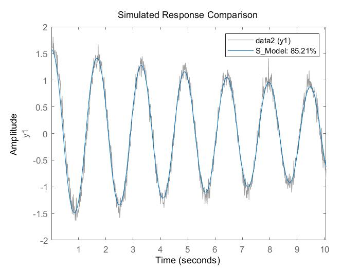
Fig. 2 Comparison between identification results and input data

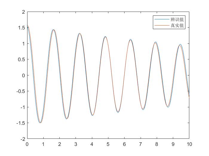
Figure 3 Comparison between identified value and real value

It can be seen that the identification accuracy is OK. At present, there are still many unknown places in the use of the relational parameter identification toolbox. We will continue to try to update it later.