Outlier detection is mainly to find some "different" data values in the data set. The so-called "different" data values mean that these data are quite different from most data. We call them "outliers", and these "outliers" are not labeled in reality, Therefore, we must automatically identify these outliers through some algorithm. We have the following definitions for outliers:
- Outliers account for a small proportion of the overall data, and the probability of generating outliers is very low.
- The characteristics of outliers are obviously different from other normal values.
data
In this blog, our data comes from the statistics of customer flow and order quantity of a foreign chain retail enterprise data , in order to make the data clearer, we only retain the following three fields:
- Date: date,
- num_people: passenger flow,
- num_order: order quantity
You can be here download Data (click download)
import pandas as pd
import numpy as np
from numpy import percentile
import matplotlib
import matplotlib.pyplot as plt
import seaborn as sns
sns.set_theme();
sns.set_style("darkgrid",{"font.sans-serif":['simhei','Droid Sans Fallback']})
from sklearn.ensemble import IsolationForest
from sklearn.preprocessing import MinMaxScaler

from pyod.models.abod import ABOD
from pyod.models.cblof import CBLOF
from pyod.models.feature_bagging import FeatureBagging
from pyod.models.hbos import HBOS
from pyod.models.iforest import IForest
from pyod.models.knn import KNN
from pyod.models.lof import LOF
from pyod.models.mcd import MCD
from pyod.models.ocsvm import OCSVM
from pyod.models.pca import PCA
from pyod.models.lscp import LSCP
import warnings
warnings.filterwarnings("ignore")
df=pd.read_csv("order_num.csv")
df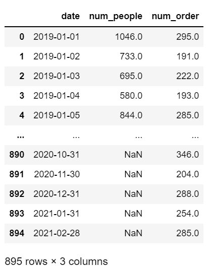
Filter missing values
In addition to outliers, there are often missing data in real data (that is, the value of some data is NaN). Generally, there are two processing methods for missing values, such as: 1 Delete the missing value directly; 2. Fill in the missing value When filling in missing values, the average value or some interpolation algorithms are generally used to insert some values in line with the historical trend of the data. Here, we use the simplest way to deal with missing data, that is, directly delete missing values. The purpose of this is to simplify the problem.
print("stay num_people Total in column %d Null values." % df['num_people'].isnull().sum())
print("stay num_order Total in column %d Null values." % df['num_order'].isnull().sum())
df=df[~df.num_people.isnull()==True]
df=df[~df.num_order.isnull()==True]
print("Total number of records after deleting missing values:",len(df))
Calculate passenger flow and order volume data distribution
print(df.num_people.describe())
print()
print(df.num_order.describe())
plt.figure(figsize=(15,8), dpi=80)
plt.subplot(221)
sns.distplot(df['num_people']);

plt.subplot(222)
sns.distplot(df['num_order']);
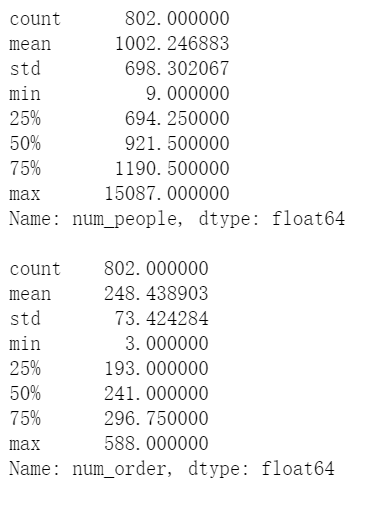
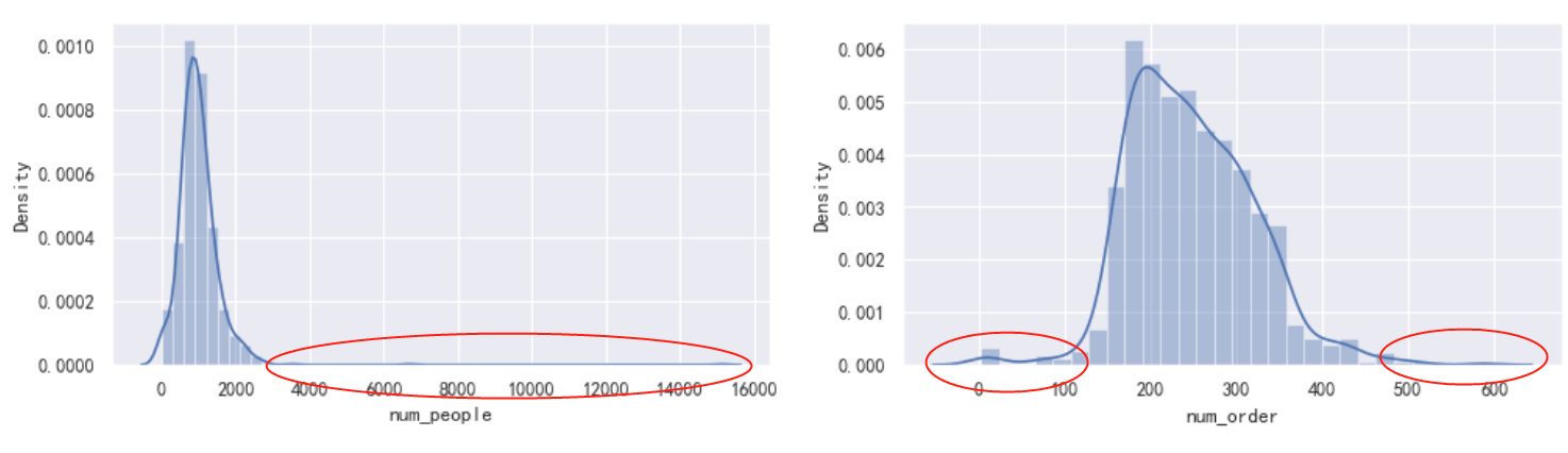
From the distribution point of view, the passenger flow (num_people) is obviously serious to the right, with a long tail on the right, and we can see that the abnormal area of the passenger flow (num_people) should be roughly distributed within the red circle in the figure above. The order quantity data presents a positive distribution, and the abnormal value area is located on the left and right sides of the distribution. Let's look at num_ Skewness and kurtosis of people. Skewness reflects the skewness of distribution, which may be left, right and long tail. Kurtosis reflects the fat and thin (width) of the shape of distribution. Please refer to this blog for specific explanations: https://blog.csdn.net/binbigdata/article/details/79897160
print("num_people's Skewness: %f" % df['num_people'].skew())
print("num_people's Kurtosis: %f " % df['num_people'].kurt())
print()
print("num_order's Skewness: %f" % df['num_order'].skew())
print("num_order's Kurtosis: %f" % df['num_order'].kurt()) 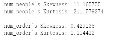
Isolationforest
IsolationForest is a simple and effective algorithm to detect outliers. It can find the area where outliers are located in the data distribution area and score all data. Those data values that fall in the abnormal area will get lower scores, while those that are not in the abnormal area will get higher scores. You can refer to this article( https://dzone.com/articles/spotting-outliers-with-isolation-forest-using-skle ). In this article, the author randomly generates two positive Pacific distributions N(-2,5) and N(2,5), finds the abnormal areas in the two distributions through the isolated forest algorithm, and generates a scoring curve. The data falling in the abnormal area will get low scores, and the data falling outside the abnormal area will get high scores:
import numpy as np
import matplotlib.pyplot as plt
x = np.concatenate((np.random.normal(loc=-2, scale=.5,size=500), np.random.normal(loc=2, scale=.5, size=500)))

isolation_forest = IsolationForest(n_estimators=100)
isolation_forest.fit(x.reshape(-1, 1))
xx = np.linspace(-6, 6, 100).reshape(-1,1)
anomaly_score = isolation_forest.decision_function(xx)
outlier = isolation_forest.predict(xx)

plt.figure(figsize=(10,8))
plt.subplot(2,1,1)
plt.hist(x)
plt.xlim([-5, 5])

plt.subplot(2,1,2)
plt.plot(xx, anomaly_score, label='Outlier score')
plt.fill_between(xx.T[0], np.min(anomaly_score), np.max(anomaly_score), where=outlier==-1, color='r', alpha=.4, label='Outlier area')
plt.legend()
plt.ylabel('Outlier score')
plt.xlabel('x')
plt.xlim([-5, 5])
plt.show() 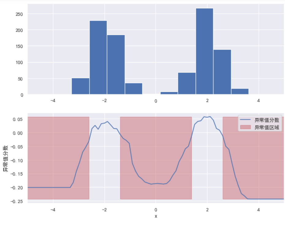
The isolated forest algorithm is used to monitor the abnormal value area of passenger flow and order volume
Isolated forest is an algorithm to detect outliers. The isolation forest algorithm is used to return the outlier score of each sample. The algorithm is based on the idea that outliers are a few data points with different characteristics. Isolated forest is a tree based model. In these trees, partitions are created by first randomly selecting features and then selecting random partition values between the minimum and maximum values of the selected features. Next, we use the isolated forest algorithm to detect the abnormal value area of passenger flow and order volume, and generate a scoring curve:
#Define isolated forest
IF1 = IsolationForest(n_estimators=100)
#Training traffic data
IF1.fit(df['num_people'].values.reshape(-1, 1))
#Split the data between the minimum and maximum passenger flow
x1 = np.linspace(df['num_people'].min(), df['num_people'].max(), len(df)).reshape(-1,1)
#Generate outlier scores for all data
anomaly_score1 = IF1.decision_function(x1)
#Predicted outliers
outlier1 = IF1.predict(x1)

IF2 = IsolationForest(n_estimators=100)
#Training order quantity data
IF2.fit(df['num_order'].values.reshape(-1, 1))
#Split data between minimum and maximum order quantities
x2 = np.linspace(df['num_order'].min(), df['num_order'].max(), len(df)).reshape(-1,1)
#Generate outlier scores for all data
anomaly_score2 = IF2.decision_function(x2)
#Predicted outliers
outlier2 = IF2.predict(x2)

plt.figure(figsize=(18,8))
plt.subplot(2,2,1)
sns.distplot(df['num_people'])

plt.subplot(2,2,2)
sns.distplot(df['num_order'])

plt.subplot(2,2,3)
plt.plot(x1, anomaly_score1, label='Outlier score')
plt.fill_between(x1.T[0], np.min(anomaly_score1), np.max(anomaly_score1),
                 where=outlier1==-1, color='r',
                 alpha=.4, label='Outlier area')
plt.legend()
plt.ylabel('Outlier score')
plt.xlabel('passenger flow(num_people)')

plt.subplot(2,2,4)
plt.plot(x2, anomaly_score2, label='Outlier score')
plt.fill_between(x2.T[0], np.min(anomaly_score2), np.max(anomaly_score2),
                 where=outlier2==-1, color='r',
                 alpha=.4, label='Outlier area')
plt.legend()
plt.ylabel('Outlier score')
plt.xlabel('Order quantity(num_order)')
plt.show(); 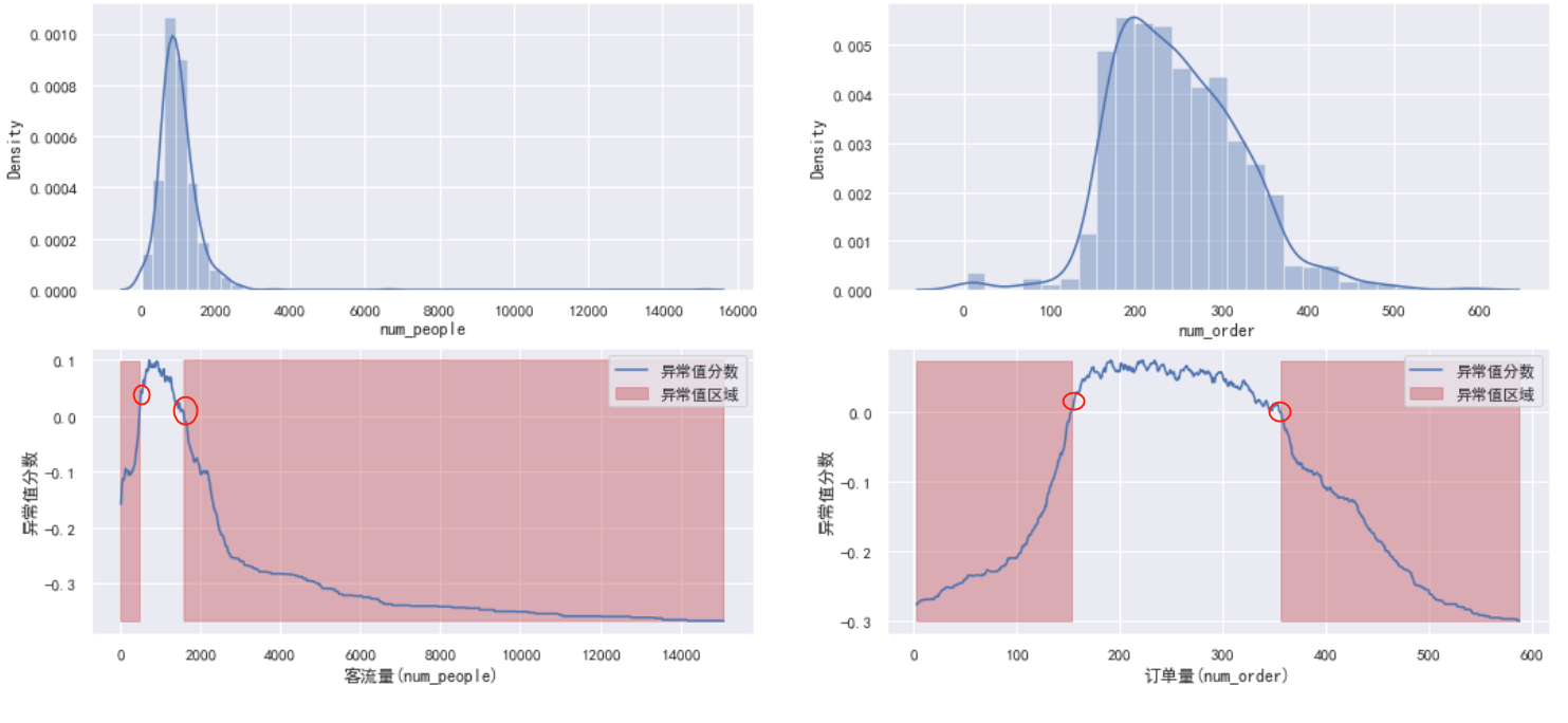
In the figure above, the isolated forest algorithm easily detects the abnormal value area of num_people and num_order, and generates a scoring curve. When the data falls within the red rectangle, it will get a lower score, and when the data falls outside the range of the red rectangle, it will get a higher score. Next, we calculate the boundary value of the outlier region of each distribution (the value in the red circle above)
x1_outlier = x1[outlier1==-1]
right_min=x1_outlier[x1_outlier>1000].min()
left_max = x1_outlier[x1_outlier<1000].max()
print('In the passenger flow abnormal value area, the maximum abnormal value on the left is:',df[df.num_people<=left_max].num_people.max())
print('The minimum abnormal value on the right in the abnormal value area of passenger flow is:',df[df.num_people>=right_min].num_people.min())
print()
x2_outlier = x2[outlier2==-1]
right_min=x2_outlier[x2_outlier>248].min()
left_max = x2_outlier[x2_outlier<248].max()
print('The maximum outliers on the left side of the order quantity outliers area are:',df[df.num_order<=left_max].num_order.max())
print('The minimum abnormal value on the right in the abnormal value area of order quantity is:',df[df.num_order>=right_min].num_order.min())
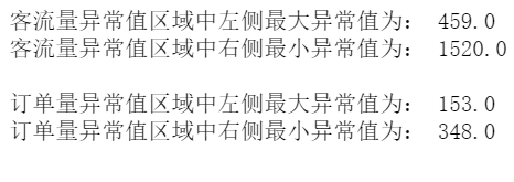
We calculated the boundary value of the abnormal value area (red area) of passenger flow and order volume respectively:
Area of abnormal passenger flow: x < = 459 and x > = 1508
Region of abnormal value of order quantity: x < = 156 and x > = 357
The above two visualization results show the outlier score and highlight the area where the outlier is located. It can be seen from the figure that the anomaly score reflects the shape of the basic distribution, and the anomaly region corresponds to the low probability region. However, so far, we have only analyzed two single variables: passenger flow and order volume. If we study carefully, we may find that some outliers determined by our model are just mathematical and statistical outliers. They may not be outliers in our business scenario. For example, in some cases, the high order volume may be caused by the high passenger flow. They may be outliers in statistical distribution, but they should not be outliers in the actual business scenario. Next, we observe the scatter distribution of the two variables of num_people and num_order at the same time, and perform linear fitting on the passenger flow and order. Those points that seriously deviate from the fitting curve can be considered as outliers. In this way, it is more in line with the actual business scenario to determine the outliers.
plt.figure(figsize=(10,6), dpi=80)
sns.regplot(data=df,x="num_people", y="num_order");
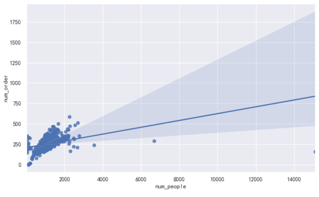
When our data is not a single variable but a multi-dimensional variable, the method of anomaly detection makes the calculation higher and mathematically more complex.
About PyOD
PyOD is a comprehensive and extensible Python toolkit for detecting abnormal objects in multidimensional data. This exciting but challenging field is often called outlier detection or anomaly detection.
PyOD includes more than 30 detection algorithms, from the classic LOF (SIGMOD 2000) to the latest COPOD (ICDM 2020). Since 2017, PyOD [aznl19] has been successfully applied to many academic research and commercial products [agsw19, alcj + 19, awdl + 19, aznhl19]. It is also widely recognized by the machine learning community and has a variety of special posts / tutorials, including Analytics Vidhya, gifts data science, KDnuggets, Computer Vision News and awesome machine learning.
PyOD official documents: https://pyod.readthedocs.io/en/latest/index.html
In this example, the following types of anomaly detection models will be used:
1. Linear model of anomaly detection
PCA: principal component analysis uses the sum of weighted projection distances to the eigenvector hyperplane as outliers (outliers)
MCD: minimum covariance determinant (using Mahalanobis distance as outlier)
OCSVM: a class of support vector machines
2. Outlier detection model based on proximity
LOF: local anomaly factor
CBLOF: local outlier factor based on Clustering
kNN: k Nearest Neighbors (use the distance to the k-th nearest neighbor as the outlier)
Median kNN outlier detection (using the median distance to k nearest neighbors as the outlier score)
HBOS: histogram based outlier score
3. Probability model of outlier detection
ABOD: angle based outlier detection
4. Anomaly checking model using integrated classifier (regression)
Isolation Forest: isolated forest
Feature Bagging: Feature Bagging
LSCP
Anomaly detection steps using PyOD
- Data scaling: standardize the passenger flow and order volume, and scale them to between 0 and 1.
- Set abnormal value proportion: set the abnormal value proportion to 1% according to experience.
- Initialize exception detection model: initialize 12 exception detection models.
- Fitting data: use the anomaly detection model to fit the data and predict the results.
- Judge abnormal value: use the threshold to judge whether the data point is a normal value or an abnormal value.
- Calculate outlier score: use the decision function to calculate the outlier score of each point.
The following code refers to "an example of comparing all implemented outlier detection models"( https://github.com/yzhao062/pyod/blob/master/notebooks/Compare%20All%20Models.ipynb )And "a great tutorial for learning exception detection in Python using PyOD library"( https://www.analyticsvidhya.com/blog/2019/02/outlier-detection-python-pyod/ )These two articles.
Scale data
Standardize the passenger flow and order volume, and scale it to between 0 and 1
#Data scaling
cols = ['num_people', 'num_order']
minmax = MinMaxScaler(feature_range=(0, 1))
print(df[cols].head())
print('--------------------------')
df[['num_people','num_order']] = minmax.fit_transform(df[cols])
print(df[cols].head())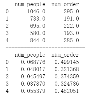
Initialize outlier detection model
Here we will initialize 12 common anomaly detection models
#Set outlier scale
outliers_fraction = 0.01

# Initialize LSCP probe set
detector_list = [LOF(n_neighbors=5), LOF(n_neighbors=10), LOF(n_neighbors=15),
                 LOF(n_neighbors=20), LOF(n_neighbors=25), LOF(n_neighbors=30),
                 LOF(n_neighbors=35), LOF(n_neighbors=40), LOF(n_neighbors=45),
                 LOF(n_neighbors=50)]
classifiers = {
    'Angle-based Outlier Detector (ABOD)':
        ABOD(contamination=outliers_fraction),
    'Cluster-based Local Outlier Factor (CBLOF)':
        CBLOF(contamination=outliers_fraction,
              check_estimator=False, random_state=0),
    'Feature Bagging':
        FeatureBagging(LOF(n_neighbors=35),
                       contamination=outliers_fraction,
                       random_state=0),
    'Histogram-base Outlier Detection (HBOS)': HBOS(
        contamination=outliers_fraction),
    'Isolation Forest': IForest(contamination=outliers_fraction,
                                random_state=0),
    'K Nearest Neighbors (KNN)': KNN(
        contamination=outliers_fraction),
    'Average KNN': KNN(method='mean',
                       contamination=outliers_fraction),
    'Local Outlier Factor (LOF)':
        LOF(n_neighbors=35, contamination=outliers_fraction),
    'Minimum Covariance Determinant (MCD)': MCD(
        contamination=outliers_fraction, random_state=0),
    'One-class SVM (OCSVM)': OCSVM(contamination=outliers_fraction),
    'Principal Component Analysis (PCA)': PCA(
        contamination=outliers_fraction, random_state=0),
    'Locally Selective Combination (LSCP)': LSCP(
        detector_list, contamination=outliers_fraction,
        random_state=0)
}

for i, clf in enumerate(classifiers.keys()):
print('Model', i + 1, clf) 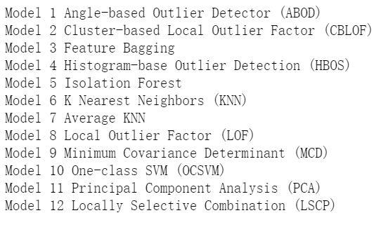
Calculate outliers
What we need to do here is to fit the data, predict the abnormal and normal data, calculate the abnormal value score, and finally visualize.
#Set num_people and num_order is merged into a two column numpy array
X1= df['num_people'].values.reshape(-1,1)
X2 = df['num_order'].values.reshape(-1,1)
X = np.concatenate((X1,X2),axis=1)
xx , yy = np.meshgrid(np.linspace(0, 1, 100), np.linspace(0, 1, 100))
plt.figure(figsize=(20, 15))
for i, (clf_name, clf) in enumerate(classifiers.items()):
#Training data
clf.fit(X)
# Predicted outlier score
scores_pred = clf.decision_function(X) * -1
# Data for predicting outliers and normal values
y_pred = clf.predict(X)
n_inliers = len(y_pred) - np.count_nonzero(y_pred)
n_outliers = np.count_nonzero(y_pred == 1)
df1 = df
df1['outlier'] = y_pred.tolist()
#Filter out num_people and num_ Normal value of order
inliers_people = np.array(df1['num_people'][df1['outlier'] == 0]).reshape(-1,1)
inliers_order = np.array(df1['num_order'][df1['outlier'] == 0]).reshape(-1,1)
#Filter out num_people and num_ Abnormal value of order
outliers_people = df1['num_people'][df1['outlier'] == 1].values.reshape(-1,1)
outliers_order = df1['num_order'][df1['outlier'] == 1].values.reshape(-1,1)
# Set a threshold to identify normal and abnormal values
threshold = np.percentile(scores_pred, 100 * outliers_fraction)
#The decision function calculates outlier scores for each data point
Z = clf.decision_function(np.c_[xx.ravel(), yy.ravel()]) * -1
Z = Z.reshape(xx.shape)
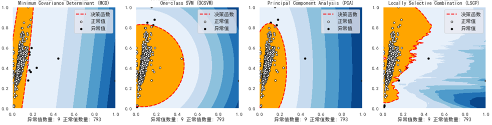
plt.subplot(3,4,i+1)
#Hierarchical coloring is performed on the graph from the minimum outlier score to the threshold
plt.contourf(xx, yy, Z, levels=np.linspace(Z.min(), threshold, 7),cmap=plt.cm.Blues_r)
#Draw a red line where the outlier score is equal to the threshold
a = plt.contour(xx, yy, Z, levels=[threshold],linewidths=2, colors='red')
#Fill the orange outline, where the anomaly score ranges from the threshold to the maximum anomaly score
plt.contourf(xx, yy, Z, levels=[threshold, Z.max()],colors='orange')
b = plt.scatter(x=inliers_people, y=inliers_order, c='white',s=20, edgecolor='k')
c = plt.scatter(x=outliers_people, y=outliers_order, c='black',s=20, edgecolor='k')
plt.axis('tight')
plt.legend([a.collections[0], b,c], ['Decision function', 'Normal value','Outliers'],
prop=matplotlib.font_manager.FontProperties(size=12),loc='upper right')
plt.xlim((0, 1))
plt.ylim((0, 1))
ss = 'Number of outliers: '+str(n_outliers)+' Number of normal values: '+str(n_inliers)
plt.title(clf_name)
plt.xlabel(ss)
plt.show(); 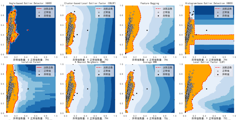
References 
CBLOF(Cluster-based Local Outlier Factor)
In CBLOF algorithm, the outlier score is calculated based on the local outlier factor of cluster group. CBLOF takes the data set and the clustering model generated by the clustering algorithm as input. It uses the parameters alpha and beta to divide the cluster into small clusters and large clusters. Then, the anomaly score is calculated based on the size of the cluster to which the point belongs and the distance to the nearest large cluster. ()
HBOS (outlier detection based on histogram) 
HBOS Assuming that the features are independent, the degree of anomaly is calculated by constructing a histogram. In multivariate anomaly detection, the histogram of each single feature can be calculated, scored separately and combined at the end.
IsolationForest (isolated forest)
The principle of isolated forest is similar to that of random forest, which is based on decision tree. Isolated forest is observed by randomly selecting features, and then isolating them according to the segmentation value between the maximum and minimum values of features. PyOD Isolation Forest module () is the wrapper of scikit learn isolation forest, which has more functions.
KNN(K - Nearest Neighbors)
Pyod for outlier detection models. knn. KNN, for data, its distance from the k-th nearest neighbor can be regarded as an outlier.
Blog post on outlier detection
Example of Comparing All Implemented Outlier Detection Models
An Awesome Tutorial to Learn Outlier Detection in Python using PyOD Library
Full code download: