Fitting, as the name suggests, is to find the mathematical relationship between data through the analysis of data. The deeper the understanding of the essence of this relationship, the higher the degree of fitting, and the clearer the relationship between data. Fitting includes linear fitting and nonlinear fitting (polynomial fitting). This paper focuses on the idea of linear fitting, because nonlinear fitting can be transformed into linear fitting through certain methods, and linear fitting has strong support in python.

We have a set of point sequences (x0, Y0), (x1, Y1), (X2, Y2) (xn,yn). If y and X are linear, which can be expressed as y=ax+b (linear equation), then fitting is to get the values of two parameters a and b. get the best a and b, so as to minimize the sum of the distances from all points in the point sequence to this line.

Complete a fitting exercise. The idea of practicing the code here is:

        1. Specify the values of a and b, that is, the model is known (it is convenient to compare the accuracy of the final results), and generate a set of data X and Y.

        2. Add noise to the data to generate sample data to be fitted.

        3. This code provides three methods to fit samples.

3.1 least square method: solve the resulting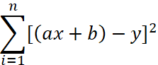Minimum a and b.

3.2 conventional equation method: solve equations in linear algebraThe weight coefficient matrix is solved θ， The result is

3.3 ￠ linear regression method: use linear regression to model this data series as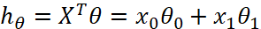=, here's the order, it is convenient to construct the matrix and calculate the offset. The X matrix in the model equation is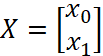, x0 and x1 are 1 and X corresponding to y=b*1+a*x. the weight coefficient matrix is，It's actually b,It's a. The loss function is solved by gradient descent methodWhen the minimum value is obtainedThe values of the matrix are the best a and b.

Select one of the three methods for fitting, and calculate the weight parameter a from the sample data_ And b_.

        4. Visualize the fitted results

import numpy as np
from sklearn.linear_model import LinearRegression
from matplotlib import pyplot as plt

SAMPLE_NUM = 100
print("Your current number of samples is:",SAMPLE_NUM)

# Preset a result first, and assume that the fitting result is y=-6x+10
X = np.linspace(-10, 10, SAMPLE_NUM)
a = -6
b = 10
Y = list(map(lambda x: a * x + b, X))
print("The standard answer is: y={}*x+{}".format(a, b))

# Increase noise, manufacturing data
Y_noise = list(map(lambda y: y + np.random.randn()*10, Y))
plt.scatter(X, Y_noise)
plt.title("data to be fitted")
plt.xlabel("x")
plt.ylabel("y")
plt.show()

A = np.stack((X, np.ones(SAMPLE_NUM)), axis=1)  # shape=(SAMPLE_NUM,2)
b = np.array(Y_noise).reshape((SAMPLE_NUM, 1))

print("The methods are listed below:"
      "1.least square method least square method "
      "2.Conventional equation method Normal Equation "
      "3.Linear regression method Linear regression")
method = int(input("Please select your fitting method: "))

Y_predict=list()
if method == 1:
    theta, _, _, _ = np.linalg.lstsq(A, b, rcond=None)
    # theta=np.polyfit(X,Y_noise,deg=1) can also be replaced by this function to fit X and y_ Noise, note that deg is the highest power of X. in the linear model y=ax+b, the highest power of X is 1
    # theta=np.linalg.solve(A,b) is not recommended
    theta = theta.flatten()
    a_ = theta[0]
    b_ = theta[1]
    print("The fitting result is: y={:.4f}*x+{:.4f}".format(a_, b_))
    Y_predict = list(map(lambda x: a_ * x + b_, X))

elif method == 2:
    AT = A.T
    A1 = np.matmul(AT, A)
    A2 = np.linalg.inv(A1)
    A3 = np.matmul(A2, AT)
    A4 = np.matmul(A3, b)
    A4 = A4.flatten()
    a_ = A4[0]
    b_ = A4[1]
    print("The fitting result is: y={:.4f}*x+{:.4f}".format(a_, b_))
    Y_predict=list(map(lambda x:a_*x+b_,X))

elif method == 3:
    # The linear regression model is used to fit the data and build the model
    model = LinearRegression()
    X_normalized = np.stack((X, np.ones(SAMPLE_NUM)), axis=1)  # shape=(50,2)
    Y_noise_normalized = np.array(Y_noise).reshape((SAMPLE_NUM, 1))  #
    model.fit(X_normalized, Y_noise_normalized)
    # The fitted model is used for prediction
    Y_predict = model.predict(X_normalized)
    # Find out a and b in the linear model y=ax+b, and confirm whether they are consistent with our setting
    a_ = model.coef_.flatten()[0]
    b_ = model.intercept_[0]
    print("The fitting result is: y={:.4f}*x+{:.4f}".format(a_, b_))

else:
    print("Please reselect")

plt.scatter(X, Y_noise)
plt.plot(X, Y_predict, c='green')
plt.title("method {}: y={:.4f}*x+{:.4f}".format(method, a_, b_))
plt.show()

The data to be fitted generated here is shown in the following figure:

The fitting results are shown in the figure below: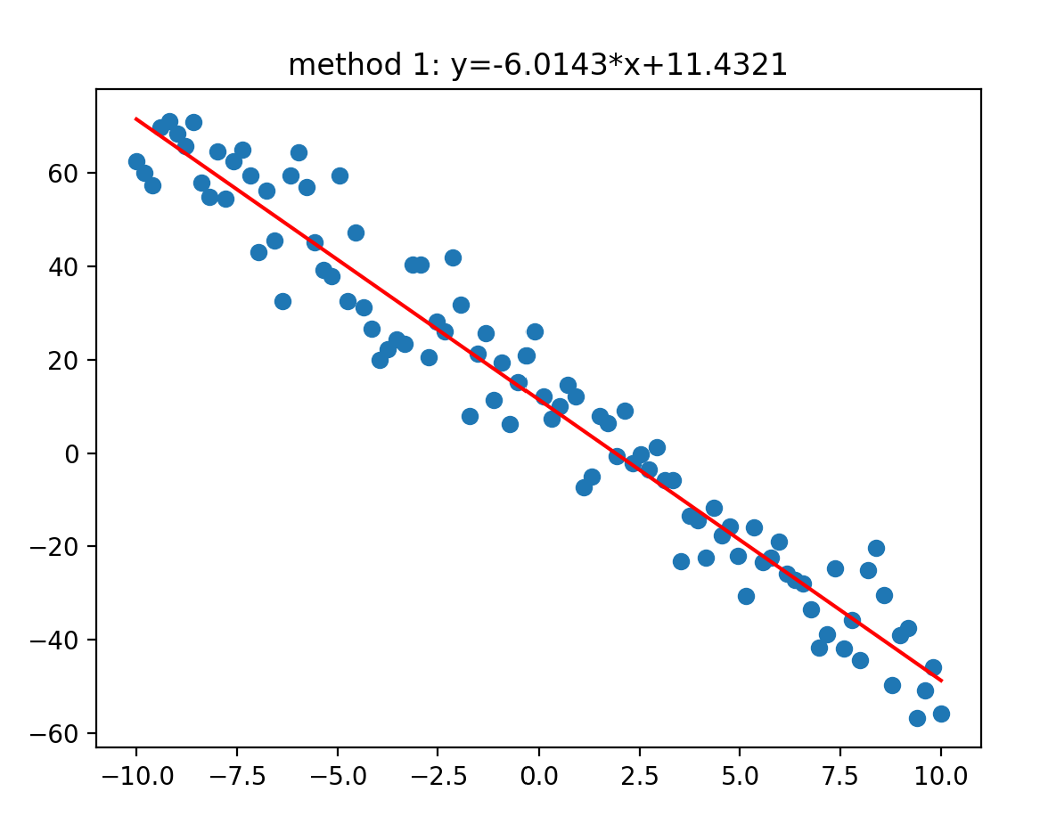

The result analysis shows that the sample generated in the code is 100 points, and the above figure is the fitting result obtained. If you want to get more accurate fitting results, you might as well set sample_ If num is a larger number, better fitting results will be obtained. I have made a group of test comparison here: it is obvious that with the increase of sample points, the fitting result is closer and closer to the standard answer of y= -6*x+10.

-6.0153

10.6758

-5.9589

10.0761

-5.9856

9.9706

-6.0021

10.0086

-6.0002

10.0002