catalogue

1. Learning objectives

2. Operation explanation

3. Job results

1. Operation 1

2. Assignment 2

1. Learning objectives

1. Using Python to achieve different investment ratios
2. Using Python to implement mean variance model

2. Operation explanation

Through the last task, you have learned something about Markowitz's mean variance portfolio model. So how do you implement it in Python? The whole process is somewhat complex, which is also quite different from the previous implementation using Excel. Therefore, we will disassemble the whole code and explain it to you one by one. In general, this code will be divided into the following main steps:

1. Collect the information of two stocks (Alibaba and New Oriental Education), mainly the daily closing prices from the beginning of 2020 to the present
2. Calculate the daily log return and daily covariance of the two stocks
3. Set different stock allocation ratios. For example, stock A increases by 5% from 0% to 100%, stock B decreases by 5% from 100% to 0%. All these different configuration ratios are recorded in A list as A comparison of the final results.
4. For each allocation proportion, calculate the comprehensive logarithmic return on investment and the uncertainty risk based on standard deviation. And record them
5. Through the chart, visualize the relationship between comprehensive income and comprehensive risk, and find the best balance point.
   For the code that has been described before, it will not be repeated here. We will only highlight the changed or newly added parts.

First, we need to collect information about Alibaba and New Oriental Education. Next, we need to try different stock proportions. To this end, we try 20 possibilities, from 0% Alibaba, 100% New Oriental Education, to 5% Alibaba, 95% New Oriental Education, and so on, to 100% Alibaba, 0% New Oriental Education. The code level will be implemented using Python loop statements.

# Try 20 different investment ratios, such as (0.0, 1.0), (0.05, 0.95), (0.95, 0.05), (1.0, 0.0)
interval = 0.05
rounds = 20
# Define the list of shareholding ratio, which is used to store 20 different investment ratios
ratio = []
# Define the list of comprehensive income, which is used to store the comprehensive income under 20 different investment ratios
combined_returns = []
# Define the list of comprehensive risks, which is used to store the comprehensive risks (standard deviation) under 20 different investment ratios
combined_risks = []

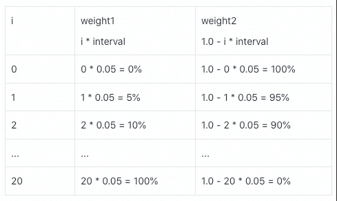
for i in range(0, rounds + 1):
    weight1 = i * interval
    weight2 = 1.0 - i * interval
    # Output current stock proportion
    print(weight1, weight2)

Among them, for i in range(0, rounds + 1) is a new cycle mode, which will produce a series of i, from 0, 1, 2,..., 20.

Note that the index starts at 0 and ends at 20 instead of 21. In this way, the proportion of the first stock is i * interval, and the proportion of the second stock is 1.0 - i * interval. In the first cycle, i=0, and the two ratios are 0% and 100% respectively. By analogy, the specific data are as follows:

Of course, you can set a smaller change interval and the corresponding combination times rounds.

In the process of circulation, for each investment proportion, we need to calculate the comprehensive income and comprehensive risk, and then use the list data structure to record it.

The specific codes are as follows:

# Add shareholding ratio to the list
    ratio.append([weight1, weight2])
    weights = np.array([weight1, weight2])
    # Calculate the expected annual comprehensive income according to the shareholding ratio
    combined_return = np.sum(weights * returns.mean()) * 250
    # Add this comprehensive income to the list
    combined_returns.append(combined_return)

    # According to the shareholding ratio, calculate the annual comprehensive standard deviation as the risk
    combined_risk = np.sqrt(np.dot(weights.T, np.dot(returns.cov() * 250, weights)))
    # Add this comprehensive income to the list
    combined_risks.append(combined_risk)

The average annual rate of return and risk calculation are used here. It should be noted that compared with the calculation of comprehensive rate of return, the calculation of comprehensive risk is a little more complex. We use the point multiplication of matrix and the transposition of matrix. Where, weights T represents the transpose of the matrix (here is the vector), NP Dot (returns. Cov() * 250, weights) dot multiplies the covariance matrix and the weight vector to make the weights T vector dot multiplication NP Dot (returns. Cov() * 250, weights). Finally, use NP The sqrt() function opens the root sign. In this step, the following formula is implemented.

The format is not as intuitive as Excel, so you need to compare it carefully. For ease of understanding, we can also use the following loop for output.

for i in range(0, len(ratio)):
    print('The stock ratio of Ali and New Oriental is', ratio[i], 'When, the comprehensive income is', combined_returns[i], '，The comprehensive risk is', combined_risks[i])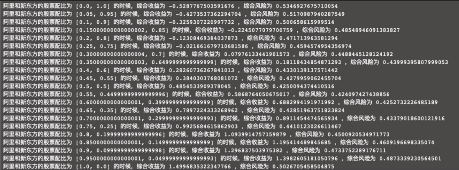

Please note that due to the precision of Python floating-point numbers, 0.15000... Or 0.64999... May occur, which actually correspond to 0.15 and 0.65 respectively.

You can also use Python for visualization and use the following code to output the scatter diagram.

combination = pd.DataFrame({'Return': combined_returns, 'Risk': combined_risks})
combination.plot(x='Risk', y='Return', kind='scatter', figsize=(10, 6))
plt.xlabel('Expected Risk')
plt.ylabel('Expected Return')
plt.show()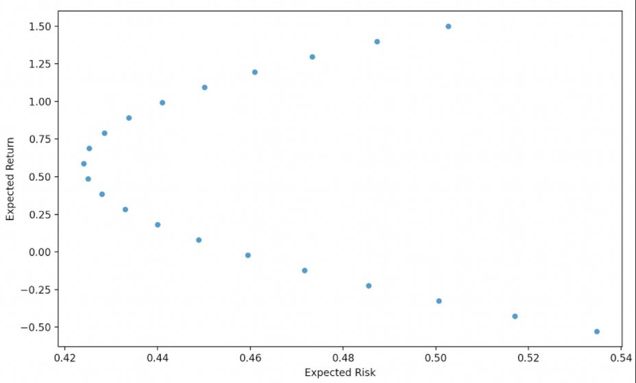

It can be seen from the results that when Alibaba, which owns 55% of the shares, and New Oriental Education, which owns 45%, we reached an equilibrium point, that is, 58.68% of the comprehensive income and 42.41% of the comprehensive risk. Of course, if the stock time period you try is different from here, the result will be different.

The complete code is listed here, which is convenient for you to read and practice.

import numpy as np
import pandas as pd
import matplotlib.pyplot as plt

# Use multiple stock codes to build a new dataframe
BABA = pd.read_csv('./BABA.csv', sep='\t', index_col=0)
EDU = pd.read_csv('./EDU.csv', sep='\t', index_col=0)

stock_data = pd.DataFrame()
stock_data['BABA'] = BABA['Adj Close']
stock_data['EDU'] = EDU['Adj Close']

# Get the daily log return of two stocks
returns = np.log(stock_data / stock_data.shift(1))
print(returns)

# Output the covariance matrix of two stocks
print(returns.cov())

# Try 20 different investment ratios, such as (0.0, 1.0), (0.05, 0.95), (0.95, 0.05), (1.0, 0.0)
interval = 0.05
rounds = 20
# Define the list of shareholding ratio, which is used to store 20 different investment ratios
ratio = []
# Define the list of comprehensive income, which is used to store the comprehensive income under 20 different investment ratios
combined_returns = []
# Define the list of comprehensive risks, which is used to store the comprehensive risks (standard deviation) under 20 different investment ratios
combined_risks = []

for i in range(0, rounds + 1):
    weight1 = i * interval
    weight2 = 1.0 - i * interval
    # Output current stock proportion
    print(weight1, weight2)

    # Add shareholding ratio to the list
    ratio.append([weight1, weight2])
    weights = np.array([weight1, weight2])
    # Calculate the expected annual comprehensive income according to the shareholding ratio
    combined_return = np.sum(weights * returns.mean()) * 250
    # Add this comprehensive income to the list
    combined_returns.append(combined_return)

    # According to the shareholding ratio, calculate the annual comprehensive standard deviation as the risk
    combined_risk = np.sqrt(np.dot(weights.T, np.dot(returns.cov() * 250, weights)))
    # Add this comprehensive income to the list
    combined_risks.append(combined_risk)

print('Stock ratio of Ali and New Oriental', ratio)
print('Comprehensive rate of return', combined_returns)
print('Comprehensive risk', combined_risks)

for i in range(0, len(ratio)):
    print('The stock ratio of Ali and New Oriental is', ratio[i], 'When, the comprehensive income is', combined_returns[i], '，The comprehensive risk is', combined_risks[i])

combination = pd.DataFrame({'Return': combined_returns, 'Risk': combined_risks})
combination.plot(x='Risk', y='Return', kind='scatter', figsize=(10, 6))
plt.xlabel('Expected Risk')
plt.ylabel('Expected Return')
plt.show()

Well, I've finished the content. It's your turn to practice. Please refer to the implementation of the above Python code to complete the following two small tasks.

• Please replace the logarithmic rate of return in the above code with a simple rate of return to see how the results of the mean variance model are different;
• After completing the previous step, please use the mean variance model to analyze the portfolio of Tencent and New Oriental Education.

While completing the exercise, please pay attention to put the screenshots of the key process and final results into a folder, package them and name them with "task 5". We have set a unified submission entry for you in the "homework" part of the project.

3. Job results

1. Operation 1

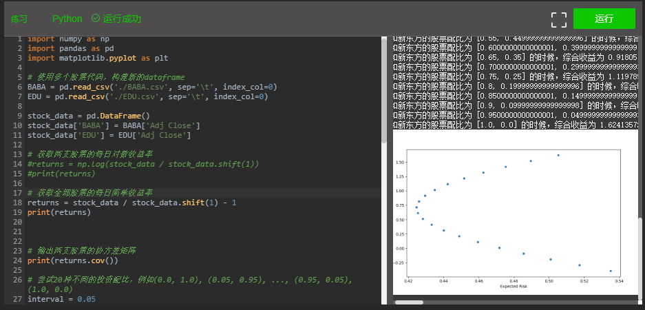
# -*- coding: utf-8 -*-
# @Software: PyCharm
# @File : Task5-1.py
# @Author : Benjamin
# @Time : 2021/9/13 11:45


import numpy as np
import pandas as pd
import matplotlib.pyplot as plt

# Use multiple stock codes to build a new dataframe
BABA = pd.read_csv('./BABA.csv', sep='\t', index_col=0)
EDU = pd.read_csv('./EDU.csv', sep='\t', index_col=0)

stock_data = pd.DataFrame()
stock_data['BABA'] = BABA['Adj Close']
stock_data['EDU'] = EDU['Adj Close']

# Get the daily log return of two stocks
#returns = np.log(stock_data / stock_data.shift(1))
#print(returns)

# Get the daily simple yield of all stocks
returns = stock_data / stock_data.shift(1) - 1
print(returns)



# Output the covariance matrix of two stocks
print(returns.cov())

# Try 20 different investment ratios, such as (0.0, 1.0), (0.05, 0.95), (0.95, 0.05), (1.0, 0.0)
interval = 0.05
rounds = 20
# Define the list of shareholding ratio, which is used to store 20 different investment ratios
ratio = []
# Define the list of comprehensive income, which is used to store the comprehensive income under 20 different investment ratios
combined_returns = []
# Define the list of comprehensive risks, which is used to store the comprehensive risks (standard deviation) under 20 different investment ratios
combined_risks = []

for i in range(0, rounds + 1):
    weight1 = i * interval
    weight2 = 1.0 - i * interval
    # Output current stock proportion
    print(weight1, weight2)

    # Add shareholding ratio to the list
    ratio.append([weight1, weight2])
    weights = np.array([weight1, weight2])
    # Calculate the expected annual comprehensive income according to the shareholding ratio
    combined_return = np.sum(weights * returns.mean()) * 250
    # Add this comprehensive income to the list
    combined_returns.append(combined_return)

    # According to the shareholding ratio, calculate the annual comprehensive standard deviation as the risk
    combined_risk = np.sqrt(np.dot(weights.T, np.dot(returns.cov() * 250, weights)))
    # Add this comprehensive income to the list
    combined_risks.append(combined_risk)

print('Stock ratio of Ali and New Oriental', ratio)
print('Comprehensive rate of return', combined_returns)
print('Comprehensive risk', combined_risks)

for i in range(0, len(ratio)):
    print('The stock ratio of Ali and New Oriental is', ratio[i], 'When, the comprehensive income is', combined_returns[i], '，The comprehensive risk is', combined_risks[i])

combination = pd.DataFrame({'Return': combined_returns, 'Risk': combined_risks})
combination.plot(x='Risk', y='Return', kind='scatter', figsize=(10, 6))
plt.xlabel('Expected Risk')
plt.ylabel('Expected Return')
plt.show()

2. Assignment 2

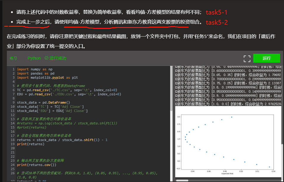
# -*- coding: utf-8 -*-
# @Software: PyCharm
# @File : Task5-2.py
# @Author : Benjamin
# @Time : 2021/9/13 11:45


import numpy as np
import pandas as pd
import matplotlib.pyplot as plt

# Use multiple stock codes to build a new dataframe
TC = pd.read_csv('./TC.csv', sep='\t', index_col=0)
EDU = pd.read_csv('./EDU.csv', sep='\t', index_col=0)

stock_data = pd.DataFrame()
stock_data['TC'] = TC['Adj Close']
stock_data['EDU'] = EDU['Adj Close']

# Get the daily log return of two stocks
#returns = np.log(stock_data / stock_data.shift(1))
#print(returns)

# Get the daily simple yield of all stocks
returns = stock_data / stock_data.shift(1) - 1
print(returns)



# Output the covariance matrix of two stocks
print(returns.cov())

# Try 20 different investment ratios, such as (0.0, 1.0), (0.05, 0.95), (0.95, 0.05), (1.0, 0.0)
interval = 0.05
rounds = 20
# Define the list of shareholding ratio, which is used to store 20 different investment ratios
ratio = []
# Define the list of comprehensive income, which is used to store the comprehensive income under 20 different investment ratios
combined_returns = []
# Define the list of comprehensive risks, which is used to store the comprehensive risks (standard deviation) under 20 different investment ratios
combined_risks = []

for i in range(0, rounds + 1):
    weight1 = i * interval
    weight2 = 1.0 - i * interval
    # Output current stock proportion
    print(weight1, weight2)

    # Add shareholding ratio to the list
    ratio.append([weight1, weight2])
    weights = np.array([weight1, weight2])
    # Calculate the expected annual comprehensive income according to the shareholding ratio
    combined_return = np.sum(weights * returns.mean()) * 250
    # Add this comprehensive income to the list
    combined_returns.append(combined_return)

    # According to the shareholding ratio, calculate the annual comprehensive standard deviation as the risk
    combined_risk = np.sqrt(np.dot(weights.T, np.dot(returns.cov() * 250, weights)))
    # Add this comprehensive income to the list
    combined_risks.append(combined_risk)

print('Stock ratio of Ali and New Oriental', ratio)
print('Comprehensive rate of return', combined_returns)
print('Comprehensive risk', combined_risks)

for i in range(0, len(ratio)):
    print('The stock ratio of Ali and New Oriental is', ratio[i], 'When, the comprehensive income is', combined_returns[i], '，The comprehensive risk is', combined_risks[i])

combination = pd.DataFrame({'Return': combined_returns, 'Risk': combined_risks})
combination.plot(x='Risk', y='Return', kind='scatter', figsize=(10, 6))
plt.xlabel('Expected Risk')
plt.ylabel('Expected Return')
plt.show()

If you think the article is good, then point a praise and a collection.

WeChat official account, and tweets later.