 https://www.jianshu.com/p/641707e4e72c
Note: when using XGBoost algorithm, you need to set X_ train,y_ The data type of Tensor type variables such as train is set to nd array type, while other algorithms can directly use Tensor data type, that is:
features = features.numpy()
labels = labels.numpy()
idx_train = idx_train.numpy()
idx_test = idx_test.numpy()
The following is the original text:
sklearn is a commonly used and easy-to-use machine learning library in python. It is very simple to summarize several commonly used machine learning algorithms. Xiaobai who wants to get started quickly can have a look~
1. Split training set and test set
from sklearn.model_selection import train_test_split
#X is the training sample; y is the label (target value); test_size is the ratio of the training set to the test set, usually 0.2 or 0.3; random_state is the seed of random number, which is actually the number of this group of random numbers. When the experiment needs to be repeated, it is guaranteed to get a group of the same random numbers. For example, if you fill in 1 every time, the random array you get is the same when other parameters are the same.
X_train, X_test, y_train, y_test = train_test_split(X, y, test_size=0.2, random_state=20)
2. logistic regression
from sklearn import linear_model
logistic = linear_model.LogisticRegression()
#If regularization is used, the parameter penalty can be added, either l1 regularization (which can more effectively resist collinearity) or l2 regularization. If it is a dataset with unbalanced categories, class can be added_ Weight parameter, which can be set or calculated by the model
logistic = linear_model.LogisticRegression( penalty='l1', class_weight='balanced')
logistic.fit(X_train,y_train)
y_pred = logistic.predict( X_test)
#If you only want to predict the probability, you can use the following function
y_pred = logistic.predict_proba(X_test)
There are two main classes related to logistic regression in sklearn: LogisticRegression and LogisticRegressionCV. Their main difference is that LogisticRegressionCV uses cross validation to select the regularization coefficient C. LogisticRegression needs to specify one regularization coefficient at a time. Except for cross validation and selection of regularization coefficient C, LogisticRegression and LogisticRegressionCV are basically used in the same way.
Many parameters of logistic regression can be debugged. Several important parameters are summarized:
- Penalty: regularization option. The selectable values of penalty are "L1" and "L2". They correspond to L1 regularization and L2 regularization respectively. The default is L2 regularization. L1 regularization can resist collinearity and also play the role of feature selection. Unimportant features will change the coefficient to 0; L2 regularization generally does not change the coefficient to 0, but it will reduce the unimportant characteristic coefficient to avoid over fitting.
The choice of penalty parameters will affect the choice of our loss function optimization algorithm. That is, the selection of parameter solver. If L2 regularization is used, five optional algorithms {Newton CG ',' lbfgs', 'liblinear', 'sag', 'saga'} can be selected. However, if penalty is L1 regularization, you can only choose 'liblinear' and 'saga'. This is because the loss function of L1 regularization is not continuously differentiable, and {'Newton CG', 'lbfgs',' sag '} these three optimization algorithms need the first-order or second-order continuous derivatives of the loss function. 'liblinear' does not have this dependency. - solver: loss function optimization method. The default is "liblinear". There are 5 methods to choose from:
a) liblinear: it is implemented using the open source liblinear library and internally uses the coordinate axis descent method to iteratively optimize the loss function.
b) lbfgs: a kind of quasi Newton method, which uses the second derivative matrix of loss function, i.e. Hessian matrix, to iteratively optimize the loss function.
c) Newton CG: it is also a kind of Newton method family. It uses the second derivative matrix of loss function, i.e. Hessian matrix, to iteratively optimize the loss function.
d) sag: random average gradient descent, which is a variant of the gradient descent method. The difference from the ordinary gradient descent method is that only a part of the samples are used to calculate the gradient in each iteration. It is suitable for very large samples.
e)saga: saga is a variant of sag. It supports L1 regularization. In many cases, the effect of saga is the best.
It can be seen from the above description that Newton CG, lbfgs and sag all need the first-order or second-order continuous derivatives of the loss function, so they can not be used for L1 regularization without continuous derivatives, but only for L2 regularization. Liblinear takes all L1 regularization and L2 regularization, but liblinear also has a limitation, that is, when selecting the classification method, it only supports ovr, multi below_ The class parameter will be explained in detail.
At the same time, sag only uses some samples for gradient iteration each time, so don't select it when the sample size is small. If the sample size is very large, such as more than 100000, sag is the first choice. However, sag cannot be used for L1 regularization, so when you have a large number of samples and need L1 regularization, you have to make your own choices. Either reduce the sample size by sampling the sample, or make feature selection in advance, or return to L2 regularization. - multi_class: the selection of classification method. There are two values: ovr and multinomial. The default is ovr.
Ovr is one vs rest (ovr), while multinomial is many vs many (MVM). If it is binary logistic regression, there is no difference between ovr and multinomial, and the difference is mainly in multiple logistic regression.
The idea of OvR is very simple. No matter how many yuan logical regression you are, we can regard it as binary logical regression. Specifically, for the classification decision of class k, we take all samples of class k as positive examples and all samples except class k as negative examples, and then do binary logistic regression above to obtain the classification model of class K. A total of T classifications are required.
MvM is relatively complex. Here is a special case of MvM, one vs one (OVO). If the model has T-class, we can select two types of samples from all T-class samples each time, which may be recorded as T1 and T2. Put all samples with T1 and T2 outputs together, take T1 as a positive example and T2 as a negative example, and carry out binary logistic regression to obtain the model parameters. We need a total of T(T-1)/2 classifications.
It can be seen from the above description that the OvR is relatively simple, but the classification effect is relatively poor (this refers to most sample distributions, and the OvR may be better under some sample distributions). MvM classification is relatively accurate, but the classification speed is not as fast as OvR.
If ovr is selected, the four loss function optimization methods liblinear, Newton CG, lbfgs and sag can be selected. However, if multinomial is selected, only Newton CG, lbfgs, saga and sag can be selected. - class_weight: various types of weights in the classification model. You can not enter, that is, the weight is not considered, or all types of weights are the same. The default is None.
If you choose to enter, you can choose balanced to let the class library calculate the type weight itself, or we can enter the weight of each type ourselves. For example, for the binary model of 0,1, we can define the class_weight={0:0.9, 1:0.1}, so the weight of type 0 is 90%, and the weight of type 1 is 10%. If class_weight if balanced is selected, the class library will calculate the weight according to the training sample size. The larger the sample size of a certain type, the lower the weight. The smaller the sample size, the higher the weight. This parameter can be adjusted to deal with class imbalance.
reference resources sklearn logistic regression (LR) class library usage summary_ sun_shengyun's column - CSDN blog
3. SVM classification
from sklearn import svm
model = svm.SVC()
model.fit(X_train, y_train)
y_pred = model.predict(X_test)
4. RandomForest classification
from sklearn.ensemble import RandomForestClassifier
#The out of bag sample is used to evaluate the quality of the model and improve the generalization ability
rf0 = RandomForestClassifier(oob_score=True)
rf0.fit(X_train,y_train)
y_pred = rf0.predict(X_test)
Random forest is also a commonly used model, which can be used for classification and regression (RandomForestRegressor is used for regression). Briefly introduce several important parameters:
- n_estimators: the number of trees in the forest. The default is 10. If there are enough resources, you can set more
- max_features: find the maximum number of features for optimal separation. The default is "auto". It is generally set to the logarithm of the feature number or the arithmetic square root of the feature number, or 40% - 50% of the feature number. This can also be used to avoid over fitting. The more the feature number, the easier it is to over fit
- max_ depth: the maximum depth of the tree. The default is None. If it is the default, the node will expand until all leaves are pure, or until all leaves are less than the min_samples_split. Over fitting can be avoided. The deeper the classification, the easier it is to over fit
- min_ samples_split: the minimum number of samples a node in the tree needs to split. The default is 2. Over fitting can be avoided. If the number of samples used for classification is too small, the model may only be suitable for the classification of samples used for training, and this problem can be avoided by using more samples. However, if the set number is too large, it may lead to under fitting, so fine tune it according to your final result
- min_ samples_leaf: the minimum number of samples required for leaf nodes in the tree. The default value is 1. It can also be used to prevent over fitting, but in case of unbalanced class problems, generally, this parameter needs to be set to a smaller value, because most of the few categories contain relatively small samples
- min_weight_fraction_leaf: and min_ samples_split is similar, except that the setting is scale, and the default is 0
- max_ leaf_ nodes: the maximum number of leaf nodes in the tree. The default is None. This is the same as Max above_ Depth may conflict, so set one when setting
5. adaboost classification
from sklearn.ensemble import AdaBoostClassifier
 #100 iterations, and the learning rate is 0.1
clf = AdaBoostClassifier(n_estimators=100,learning_rate=0.1)
clf.fit(X_train,y_train)
y_pred = clf.predict( X_test)
6. GBDT classification
from sklearn.ensemble import GradientBoostingClassifier
 #100 iterations, and the learning rate is 0.1
clf = GradientBoostingClassifier(n_estimators=100, learning_rate=0.1)
clf.fit(X_train,y_train)
y_pred = clf.predict( X_test)
7. Neural network
from sklearn import linear_model
from sklearn.neural_network import BernoulliRBM
from sklearn.pipeline import Pipeline
logistic = linear_model.LogisticRegression()
rbm = BernoulliRBM(random_state=0, verbose=True)
classifier = Pipeline(steps=[('rbm', rbm), ('logistic', logistic)])
rbm.learning_rate = 0.1
rbm.n_iter = 20
rbm.n_components = 100
#Regularization strength parameter
logistic.C = 1000
classifier.fit(X_train, y_train)
y_pred = classifier.predict(X_test)
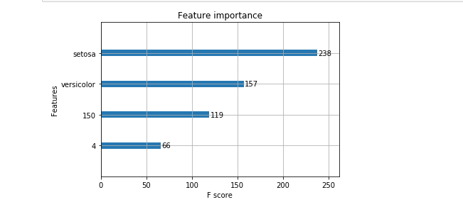
8. XGboost
from xgboost import XGBClassifier
from matplotlib import pyplot
model = XGBClassifier()
model.fit(X_train,y_train)
y_pred = model.predict(X_test)
#View forecast accuracy
accuracy_score(y_test, y_pred)
#Importance of drawing features
from xgboost import plot_importance
plot_importance(model)
pyplot.show()
9. Ridge regression
Ridge regression compresses the coefficients by adding a regular term (L2 norm) on the basis of RSS (residual sum of squares, otherwise known as SSE (Sum of Squares for Error)) of ordinary least squares linear regression, so as to avoid over fitting and collinearity.
Although the coefficient is small, it can effectively reduce the variance, but the coefficient cannot be guaranteed to be 0, so there is still a long string of characteristics, which will make the model difficult to explain. This is the disadvantage of ridge regression.
# Ridge regression
from sklearn import linear_model
X = [[0, 0], [1, 1], [2, 2]]
y = [0, 1, 2]
clf = linear_model.Ridge(alpha=0.1)  # Set regularization strength
clf.fit(X, y)  # Parameter fitting
print(clf.coef_)  # coefficient
print(clf.intercept_)  # Constant coefficient
print(clf.predict([[3, 3]]))  # Calculate the predicted value
print(clf.decision_function(X))  # Prediction is the same as predict
print(clf.score(X, y))  # R^2, goodness of fit
print(clf.get_params())  # Get parameter information
print(clf.set_params(fit_intercept=False))  # Reset the parameters. For example, set whether to use intercept to false, that is, intercept is not used.
10. Lasso regression
Lasso compresses the coefficients by adding a regular term (L1 norm) to the RSS of ordinary least squares linear regression, so as to avoid over fitting and collinearity.
The coefficient of Lasso regression can be 0, which can play a real feature screening effect.
# Lasso regression
from sklearn import linear_model
X = [[0, 0], [1, 1], [2, 2]]
y = [0, 1, 2]
clf = linear_model.Lasso(alpha=0.1)  # Set regularization strength
clf.fit(X, y)  # Parameter fitting
print(clf.coef_)  # coefficient
print(clf.intercept_)  # Constant coefficient
print(clf.predict([[3, 3]]))  # Calculate the predicted value
print(clf.decision_function(X))  # Prediction is the same as predict
print(clf.score(X, y))  # R^2, goodness of fit
print(clf.get_params())  # Get parameter information
print(clf.set_params(fit_intercept=False))  # Reset the parameters. For example, set whether to use intercept to false, that is, intercept is not used.
11. Parameter adjustment
Each classification or regression has many parameters that can be set. How many should these be set to be more appropriate? sklearn also has a module that can help us set a better parameter. This module is called GridSearchCV. Next, use adaboost algorithm and iris data set to find the best learning_rate as an example.
from sklearn.model_selection import GridSearchCV
from sklearn.model_selection import StratifiedKFold
learning_rate = [0.0001, 0.001, 0.01, 0.1, 0.2, 0.3]
model = AdaBoostClassifier()
param_grid = dict(learning_rate=learning_rate)
#Set 10 fold cross validation
kfold = StratifiedKFold(n_splits=10, shuffle=True)
grid_search = GridSearchCV(model, param_grid, scoring="neg_log_loss", n_jobs=-1, cv=kfold)
grid_result = grid_search.fit( iris, iris_y)
#Print the best learning_rate
print("Best: %f using %s" % (grid_result.best_score_, grid_result.best_params_))
Out[349]: Best: -0.160830 using {'learning_rate': 0.3}
#Among the six learning rates given, the best learning rate is 0.3
#Other parameters can also be printed
means = grid_result.cv_results_['mean_test_score']
stds = grid_result.cv_results_['std_test_score']
params = grid_result.cv_results_['params']
for mean, stdev, param in zip(means, stds, params):
    print("%f (%f) with: %r" % (mean, stdev, param))
Out[350]:-0.462098 (0.000000) with: {'learning_rate': 0.0001}
-0.347742 (0.106847) with: {'learning_rate': 0.001}
-0.237053 (0.056082) with: {'learning_rate': 0.01}
-0.184642 (0.085079) with: {'learning_rate': 0.1}
-0.163586 (0.117306) with: {'learning_rate': 0.2}
-0.160830 (0.135698) with: {'learning_rate': 0.3}
12. Check the result accuracy, confusion matrix, auc, etc
from sklearn.metrics import accuracy_score
from sklearn.metrics import roc_auc_score
from sklearn.metrics import confusion_matrix
#Calculation accuracy
accuracy = accuracy_score(y_test, y_pred)
#Computing auc is generally aimed at two kinds of classification problems
auc = roc_auc_score(y_test, y_pred)
#Computing confusion matrix is generally aimed at two kinds of classification problems
conMat = confusion_matrix(y_test, y_pred)
Author: Xiao Han_ Xiao Hong
Link: https://www.jianshu.com/p/641707e4e72c
Source: Jianshu
The copyright belongs to the author. For commercial reprint, please contact the author for authorization, and for non-commercial reprint, please indicate the source.