preface
This competition is a data analysis novice learner development competition organized by Tianchi data platform. The content of the competition is used car price prediction. The data is provided by Tianchi platform. When I first saw this topic, my first reaction was to use the linear regression method. Of course, this is the simplest, and the possible results are not particularly good. Therefore, we use lgb here, Let's have a look
Tip: the following is the main content of this article. The following cases can be used for reference
1, Game question understanding
1.1 overview of competition questions
The competition requires the contestants to establish a model and the transaction price of second-hand cars according to the given data set.
The task of the competition is to predict the transaction price of second-hand cars. The data set can be seen and downloaded after registration. The data comes from the second-hand car transaction record of A trading platform. The total amount of data is more than 40w, including 31 columns of variable information, of which 15 are anonymous variables. In order to ensure the fairness of the competition, 150000 will be selected as the training set, 50000 as the test set A and 50000 as the test set B. at the same time, the information such as name, model, brand and regionCode will be desensitized.
1.2 prediction indicators
The evaluation standard of this competition is MAE(Mean Absolute Error):
M
A
E
=
∑
i
=
1
n
∣
y
i
−
y
^
i
∣
n
MAE=\frac{\sum_{i=1}^{n}\left|y_{i}-\hat{y}_{i}\right|}{n}
MAE=n Σ i=1n ∣ yi − y ^ i ∣ where
y
i
y_{i}
yi represents the third party
i
i
The true value of i samples, where
y
^
i
\hat{y}_{i}
y ^ i stands for the second
i
i
Predicted value of i samples.
Description of evaluation indicators of general problems:
What are the evaluation indicators:
The evaluation index is our numerical quantification of the effect of a model. (it's a bit similar to scoring a commodity evaluation, which is a score between the model effect and the ideal effect)
Generally speaking, the evaluation indicators of classification and regression problems have the following forms:
Common evaluation indicators of classification algorithm are as follows:
- For class II classifiers / classification algorithms, the main evaluation indicators are accuracy,
[Precision, Recall, F-score, Pr curve], ROC-AUC curve. - For multi class classifiers / classification algorithms, the main evaluation indicators are accuracy, [macro average and micro average, F-score].
Common evaluation indicators for regression prediction are as follows:
- Mean Absolute Error (MAE), mean square error (MSE), Mean Absolute Percentage Error (MAPE), root mean square error (root mean square error), R2 (R-Square)
Mean Absolute Error (MAE): Mean Absolute Error, which can better reflect the actual situation of the error between the predicted value and the real value. Its calculation formula is as follows: M A E = 1 N ∑ i = 1 N ∣ y i − y ^ i ∣ MAE=\frac{1}{N} \sum_{i=1}^{N}\left|y_{i}-\hat{y}_{i}\right| MAE=N1i=1∑N∣yi−y^i∣
Mean square error (MSE), mean square error, its calculation formula is: M S E = 1 N ∑ i = 1 N ( y i − y ^ i ) 2 MSE=\frac{1}{N} \sum_{i=1}^{N}\left(y_{i}-\hat{y}_{i}\right)^{2} MSE=N1i=1∑N(yi−y^i)2
The formula of R2(R-Square) is: sum of squares of residuals: S S r e s = ∑ ( y i − y ^ i ) 2 SS_{res}=\sum\left(y_{i}-\hat{y}{i}\right)^{2} SSres = ∑ (yi − y ^ i)2 total average: S S t o t = ∑ ( y i − y ‾ i ) 2 SS{tot}=\sum\left(y_{i}-\overline{y}_{i}\right)^{2} SStot=∑(yi−yi)2
among y ‾ \overline{y} y represents y y The average value of y R 2 R^2 R2 expression is: R 2 = 1 − S S r e s S S t o t = 1 − ∑ ( y i − y ^ i ) 2 ∑ ( y i − y ‾ ) 2 R^{2}=1-\frac{SS_{res}}{SS_{tot}}=1-\frac{\sum\left(y_{i}-\hat{y}{i}\right)^{2}}{\sum\left(y{i}-\overline{y}\right)^{2}} R2=1−SStotSSres=1−∑(yi−y)2∑(yi−y^i)2 R 2 R^2 R2 is used to measure the proportion of the variation of dependent variables that can be explained by independent variables. The value range is 0 ~ 1, R 2 R^2 The closer R2 is to 1, the greater the proportion of the sum of squares in the total sum of squares, the closer the regression line is to each observation point, the more the change of y value is explained by the change of x, and the better the fitting degree of regression is. therefore R 2 R^2 R2 is also known as the statistic of Goodness of Fit.
y i y_{i} yi represents the true value, y ^ i \hat{y}{i} y ^ i represents the predicted value, y ‾ i \overline{y}{i} y i represents the sample mean value. The higher the score, the better the fitting effect.
2, baseline
1. Import and storage
import numpy as np
import pandas as pd
import warnings
import matplotlib
import matplotlib.pyplot as plt
import seaborn as sns
from scipy.special import jn
from IPython.display import display, clear_output
import time

warnings.filterwarnings('ignore')
%matplotlib inline

## Model predicted
from sklearn import linear_model
from sklearn import preprocessing
from sklearn.svm import SVR
from sklearn.ensemble import RandomForestRegressor,GradientBoostingRegressor

## Data dimensionality reduction processing
from sklearn.decomposition import PCA,FastICA,FactorAnalysis,SparsePCA

import lightgbm as lgb
import xgboost as xgb

## Parameter search and evaluation
from sklearn.model_selection import GridSearchCV,cross_val_score,StratifiedKFold,train_test_split
from sklearn.metrics import mean_squared_error, mean_absolute_error
2. Read in data
The code is as follows (example):
## Read data through pandas (pandas is a very friendly data reading function library)
Train_data = pd.read_csv('C:\\Users\\TINKPAD\\Desktop\\python_work\\kaggle\Used car transaction price forecast\\used_car_train_20200313.csv', sep=' ')
TestA_data = pd.read_csv('C:\\Users\\TINKPAD\\Desktop\\python_work\\kaggle\Used car transaction price forecast\\used_car_testB_20200421.csv', sep=' ')

## Size information of output data
print('Train data shape:',Train_data.shape)
print('TestA data shape:',TestA_data.shape)
Train data shape: (150000, 31)
TestA data shape: (50000, 30)
## Pass head() briefly browses the form of the read data
Train_data.head()
   SaleID    name   regDate  model  ...      v_11      v_12      v_13      v_14
0       0     736  20040402   30.0  ...  2.804097 -2.420821  0.795292  0.914762
1       1    2262  20030301   40.0  ...  2.096338 -1.030483 -1.722674  0.245522
2       2   14874  20040403  115.0  ...  1.803559  1.565330 -0.832687 -0.229963
3       3   71865  19960908  109.0  ...  1.285940 -0.501868 -2.438353 -0.478699
4       4  111080  20120103  110.0  ...  0.910783  0.931110  2.834518  1.923482

[5 rows x 31 columns]
## Pass info() briefly shows the corresponding data column names and the missing information of NAN
Train_data.info()
<class 'pandas.core.frame.DataFrame'>
RangeIndex: 150000 entries, 0 to 149999
Data columns (total 31 columns):
 #   Column             Non-Null Count   Dtype
---  ------             --------------   -----
 0   SaleID             150000 non-null  int64
 1   name               150000 non-null  int64
 2   regDate            150000 non-null  int64
 3   model              149999 non-null  float64
 4   brand              150000 non-null  int64
 5   bodyType           145494 non-null  float64
 6   fuelType           141320 non-null  float64
 7   gearbox            144019 non-null  float64
 8   power              150000 non-null  int64
 9   kilometer          150000 non-null  float64
 10  notRepairedDamage  150000 non-null  object
 11  regionCode         150000 non-null  int64
 12  seller             150000 non-null  int64
 13  offerType          150000 non-null  int64
 14  creatDate          150000 non-null  int64
 15  price              150000 non-null  int64
 16  v_0                150000 non-null  float64
 17  v_1                150000 non-null  float64
 18  v_2                150000 non-null  float64
 19  v_3                150000 non-null  float64
 20  v_4                150000 non-null  float64
 21  v_5                150000 non-null  float64
 22  v_6                150000 non-null  float64
 23  v_7                150000 non-null  float64
 24  v_8                150000 non-null  float64
 25  v_9                150000 non-null  float64
 26  v_10               150000 non-null  float64
 27  v_11               150000 non-null  float64
 28  v_12               150000 non-null  float64
 29  v_13               150000 non-null  float64
 30  v_14               150000 non-null  float64
dtypes: float64(20), int64(10), object(1)
memory usage: 35.5+ MB
## Pass columns view column names
Train_data.columns
Index(['SaleID', 'name', 'regDate', 'model', 'brand', 'bodyType', 'fuelType',
       'gearbox', 'power', 'kilometer', 'notRepairedDamage', 'regionCode',
       'seller', 'offerType', 'creatDate', 'price', 'v_0', 'v_1', 'v_2', 'v_3',
       'v_4', 'v_5', 'v_6', 'v_7', 'v_8', 'v_9', 'v_10', 'v_11', 'v_12',
       'v_13', 'v_14'],
      dtype='object')
## Pass describe() can view some statistical information of the numerical characteristic column
Train_data.describe()
3. Feature and label construction
numerical_cols = Train_data.select_dtypes(exclude = 'object').columns
print(numerical_cols)
Index(['SaleID', 'name', 'regDate', 'model', 'brand', 'bodyType', 'fuelType',
       'gearbox', 'power', 'kilometer', 'regionCode', 'seller', 'offerType',
       'creatDate', 'price', 'v_0', 'v_1', 'v_2', 'v_3', 'v_4', 'v_5', 'v_6',
       'v_7', 'v_8', 'v_9', 'v_10', 'v_11', 'v_12', 'v_13', 'v_14'],
      dtype='object')
categorical_cols = Train_data.select_dtypes(include = 'object').columns
print(categorical_cols)
Index(['notRepairedDamage'], dtype='object')
##2) Build training and test samples
## Select feature column
feature_cols = [col for col in numerical_cols if col not in ['SaleID','name','regDate','creatDate','price','model','brand','regionCode','seller']]
feature_cols = [col for col in feature_cols if 'Type' not in col]

## Training sample column, training sample column and feature column
X_data = Train_data[feature_cols]
Y_data = Train_data['price']

X_test  = TestA_data[feature_cols]

print('X train shape:',X_data.shape)
print('X test shape:',X_test.shape)
X train shape: (150000, 18)
X test shape: (50000, 18)
## A statistical function is defined to facilitate subsequent information statistics
def Sta_inf(data):
    print('_min',np.min(data))
    print('_max:',np.max(data))
    print('_mean',np.mean(data))
    print('_ptp',np.ptp(data))
    print('_std',np.std(data))
    print('_var',np.var(data))
##3) Basic distribution information of statistical labels
print('Sta of label:')
Sta_inf(Y_data)
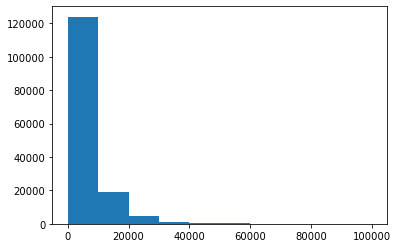
Sta of label:
_min 11
_max: 99999
_mean 5923.327333333334
_ptp 99988
_std 7501.973469876438
_var 56279605.94272992
## Draw the statistical chart of labels and view the distribution of labels
plt.hist(Y_data)
plt.show()
plt.close()
##4) The default value is filled with - 1
X_data = X_data.fillna(-1)
X_test = X_test.fillna(-1)
4. Model training and prediction
##1) Use xgb for 50% cross validation to check the parameter effect of the model
## xgb-Model
xgr = xgb.XGBRegressor(n_estimators=120, learning_rate=0.1, gamma=0, subsample=0.8,\
        colsample_bytree=0.9, max_depth=7) #,objective ='reg:squarederror'

scores_train = []
scores = []

## 5-fold cross validation method
sk=StratifiedKFold(n_splits=5,shuffle=True,random_state=0)
for train_ind,val_ind in sk.split(X_data,Y_data):

    train_x=X_data.iloc[train_ind].values
    train_y=Y_data.iloc[train_ind]
    val_x=X_data.iloc[val_ind].values
    val_y=Y_data.iloc[val_ind]

    xgr.fit(train_x,train_y)
    pred_train_xgb=xgr.predict(train_x)
    pred_xgb=xgr.predict(val_x)

    score_train = mean_absolute_error(train_y,pred_train_xgb)
    scores_train.append(score_train)
    score = mean_absolute_error(val_y,pred_xgb)
    scores.append(score)

print('Train mae:',np.mean(score_train))
print('Val mae',np.mean(scores))
Train mae: 622.836567743063
Val mae 714.0856746034109
##2) Define xgb and lgb model functions
def build_model_xgb(x_train,y_train):
    model = xgb.XGBRegressor(n_estimators=150, learning_rate=0.1, gamma=0, subsample=0.8,\
        colsample_bytree=0.9, max_depth=7) #, objective ='reg:squarederror'
    model.fit(x_train, y_train)
    return model

def build_model_lgb(x_train,y_train):
    estimator = lgb.LGBMRegressor(num_leaves=127,n_estimators = 150)
    param_grid = {
        'learning_rate': [0.01, 0.05, 0.1, 0.2],
    }
    gbm = GridSearchCV(estimator, param_grid)
    gbm.fit(x_train, y_train)
    return gbm
##3) The segmentation data set (Train,Val) is used for model training, evaluation and prediction
## Split data with val
x_train,x_val,y_train,y_val = train_test_split(X_data,Y_data,test_size=0.3)
print('Train lgb...')
model_lgb = build_model_lgb(x_train,y_train)
val_lgb = model_lgb.predict(x_val)
MAE_lgb = mean_absolute_error(y_val,val_lgb)
print('MAE of val with lgb:',MAE_lgb)
Train lgb...
MAE of val with lgb: 691.2926210859479
print('Predict lgb...')
model_lgb_pre = build_model_lgb(X_data,Y_data)
subA_lgb = model_lgb_pre.predict(X_test)
print('Sta of Predict lgb:')
Sta_inf(subA_lgb)
Predict lgb...
Sta of Predict lgb:
_min -589.8793550785414
_max: 90760.26063584947
_mean 5906.935218383807
_ptp 91350.13999092802
_std 7344.644970956768
_var 53943809.749400534
print('Train xgb...')
model_xgb = build_model_xgb(x_train,y_train)
val_xgb = model_xgb.predict(x_val)
MAE_xgb = mean_absolute_error(y_val,val_xgb)
print('MAE of val with xgb:',MAE_xgb)
Train xgb...
MAE of val with xgb: 715.2890582658079
Predict xgb...
Sta of Predict xgb:
_min -318.20892
_max: 90140.625
_mean 5910.7607
_ptp 90458.836
_std 7345.965
_var 53963196.0
##4) The results of the two models are weighted and fused
## Here we adopt a simple weighted fusion method
val_Weighted = (1-MAE_lgb/(MAE_xgb+MAE_lgb))*val_lgb+(1-MAE_xgb/(MAE_xgb+MAE_lgb))*val_xgb
val_Weighted[val_Weighted<0]=10 # Since we found that the predicted minimum value has a negative number, but in the real case, if the price is negative, it does not exist, so we made the corresponding post correction
print('MAE of val with Weighted ensemble:',mean_absolute_error(y_val,val_Weighted))
sub_Weighted = (1-MAE_lgb/(MAE_xgb+MAE_lgb))*subA_lgb+(1-MAE_xgb/(MAE_xgb+MAE_lgb))*subA_xgb
MAE of val with Weighted ensemble: 689.3545169592032
## View statistics of predicted values
plt.hist(Y_data)
plt.show()
plt.close()

##5) Output results
sub = pd.DataFrame()
sub['SaleID'] = TestA_data.SaleID
sub['price'] = sub_Weighted
sub.to_csv('./sub_Weighted.csv',index=False)
sub.head()
   SaleID        price
0  200000  1177.369198
1  200001  1806.742061
2  200002  8560.577630
3  200003  1346.459235
4  200004  2074.334952
Final score:

summary
From this baseline, we can see that the prediction results are obtained by using the weighted fusion of the two models, and the final score is higher, which also shows that the above code has a lot of room for progress