brief introduction

On the previous blog: Introduction to CNN network in the introduction series of data mining (11.5) In this blog, we will use code to explain how to use keras to build a CNN network to train CIFAR-10 dataset.

If you are not familiar with keras, you can take a look Official documents . Or take a look at my previous blog: Introduction to keras and construction of DNN network to recognize MNIST In this blog, we use keras to build a DNN network, and give an introduction to keras.

CIFAR-10 data set

CIFAR-10 data set is a set of images, which is usually used to train machine learning and computer vision algorithms. It is one of the widely used data sets in machine learning research. The CIFAR-10 dataset contains a total of 6w 32x32 color images of 10 different categories. There are 10 different categories representing airplanes, cars, birds, cats, deer, dogs, frogs, horses, ships and trucks. 6000 images per category

These datasets are provided in keras. The code to load the dataset is as follows:

from keras.datasets import cifar10

(x_train, y_train), (x_test, y_test) = cifar10.load_data()

print(x_train.shape, 'x_train samples')
print(x_test.shape, 'x_test samples')
print(y_train.shape, 'y_trian samples')
print(y_test.shape, 'Y_test samples')

The output results are as follows:

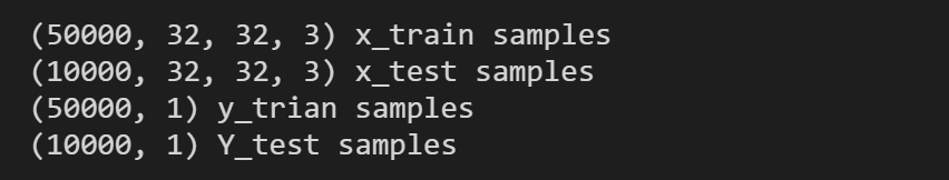
There are 5w pictures in the training set and 1w pictures in the test set. In the \ (x \) data set, the picture is \ ((32, 32, 3) \), which means the picture size is \ (32 \times 32 \), which is a picture of 3 channels (R,G,B).

Show picture content

We can show the content of the picture a little. The python code is as follows:

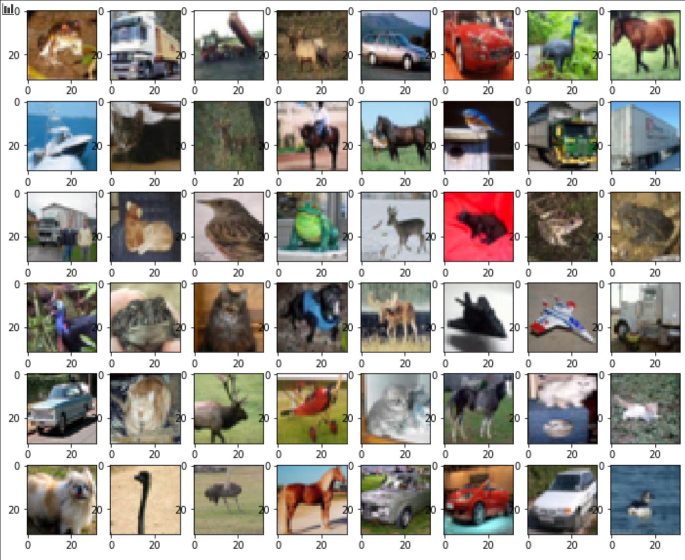
import matplotlib.pyplot as plt
%matplotlib inline

plt.figure(figsize=(12,10))
x, y = 8, 6

for i in range(x*y):  
    plt.subplot(y, x, i+1)
    plt.imshow(x_train[i],interpolation='nearest')
plt.show()

Here are some pictures in the dataset:

Dataset transformation

Similarly, we need to encode the class tag with one hot code:

import keras
# Convert class vector to binary class matrix.
y_train = keras.utils.to_categorical(y_train, 10)
y_test = keras.utils.to_categorical(y_test, 10)

In fact, in this step, there are still many bull (SAO) operations, such as data set enhancement, transformation, etc., which can improve the robustness of the model to a certain extent and prevent over fitting. Here, we just need to do one-hot coding for the data set labels.

Building CNN network

The network model code is as follows:

from keras.models import Sequential
from keras.layers import Dense, Dropout, Activation, Flatten,Conv2D, MaxPooling2D

# Building CNN network
model = Sequential()

# Add volume layer
model.add(Conv2D(32, (3, 3), padding='same',input_shape=x_train.shape[1:]))
# Add active layer
model.add(Activation('relu'))
model.add(Conv2D(32, (3, 3)))
model.add(Activation('relu'))

# Add maximum pooling layer
model.add(MaxPooling2D(pool_size=(2, 2)))
model.add(Dropout(0.25))

model.add(Conv2D(64, (3, 3), padding='same'))
model.add(Activation('relu'))
model.add(Conv2D(64, (3, 3)))
model.add(Activation('relu'))
model.add(MaxPooling2D(pool_size=(2, 2)))
model.add(Dropout(0.25))

# Change the output data of the previous layer into one dimension
model.add(Flatten())
# Add full connection layer
model.add(Dense(512))
model.add(Activation('relu'))
model.add(Dropout(0.5))
model.add(Dense(10))
model.add(Activation('softmax'))

# Introduction of network model
print(model.summary())

Here is the code:

Conv2D

Conv2D represents the convolution layer of 2D. Maybe someone here will ask, isn't my picture RGB? Why Conv2D is used instead of Conv3D. First of all, this "2" in Conv2D represents that the convolution layer can be moved in two dimensions (i.e. width,length). Similarly, "3" in Conv3D means that the convolution layer can be moved in three dimensions (such as width,length, time in video). So for RGB, the number of channels in the convolution process is the number of channels in the filter (convolution kernel).

To put it simply:

input

Convolutional kernel filter

It is worth noting that the result after convolution is two-dimensional. (because the result of 3D convolution will be added)

Then continue to explain the parameters of Conv2D:

Conv2D(32, (3, 3), padding='same',input_shape=x_train.shape[1:])

• 32 represents the dimension of the output space (that is, the number of outputs of the filter)
• (3, 3) represents the size of convolution kernel
• Strips (not used here): This represents the sliding step size.
• input_shape: the dimension of input, here is (28,28,3)

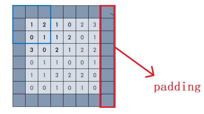
As mentioned in the previous blog, padding has two values in keras: "valid" or "same" (case sensitive).

• valid padding: only the original image is used without any processing, and the convolution kernel is not allowed to exceed the original image boundary
• same padding: filling, allowing the convolution kernel to exceed the original image boundary, and making the size of the convolution result consistent with the original

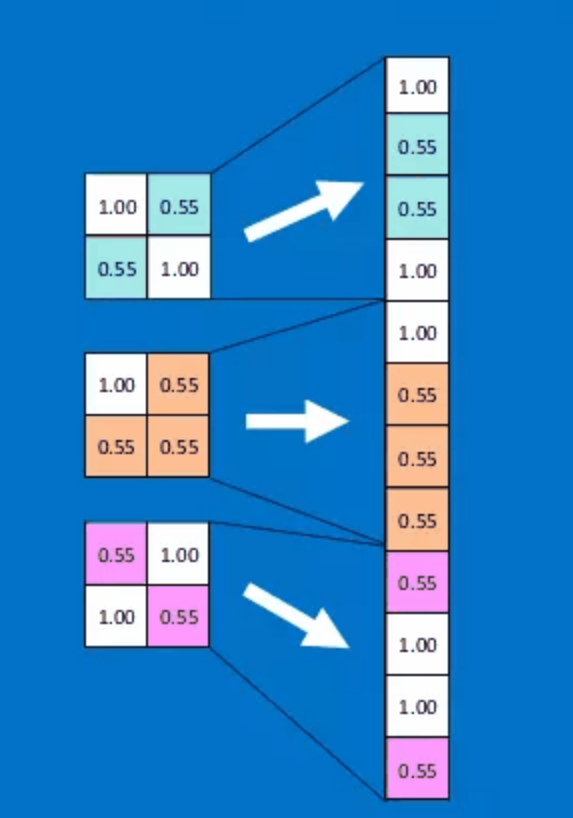
Flatten

The Flatten layer is to transform multidimensional data into one-dimensional data:

Building the network

from keras.optimizers import RMSprop
# Use RMSprop to train the model.
model.compile(loss='categorical_crossentropy',
              optimizer=RMSprop(),
              metrics=['accuracy']
             )

The other parameters have been mentioned in the last two blogs, so we will not repeat them.

Conduct training assessment

Here, you can adjust the size of the batch size according to your computer configuration.

history = model.fit(x_train, y_train,
                    batch_size=32,
                    epochs=64,
                    verbose=1,
                    validation_data=(x_test, y_test)
                   )

In the case of i5-10 generation u, mx250, a round of training will take about 27s.

After training, evaluate:

score = model.evaluate(x_test, y_test, verbose=0)
print('Test loss:', score[0])
print('Test accuracy:', score[1])

The results are as follows:

This result can be said to be inexhaustible, 😔.

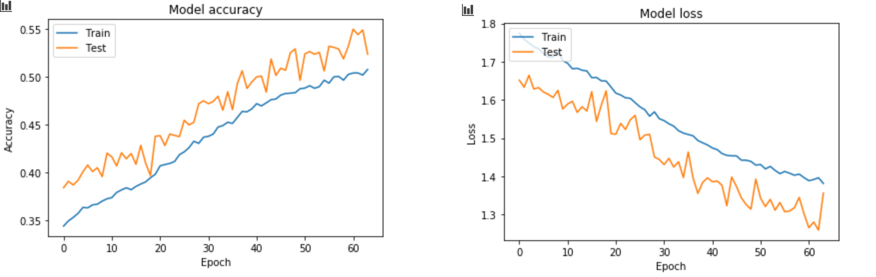
View training history

import matplotlib.pyplot as plt

# Draw the accuracy value of training set and test set in the training process
plt.plot(history.history['accuracy'])
plt.plot(history.history['val_accuracy'])
plt.title('Model accuracy')
plt.ylabel('Accuracy')
plt.xlabel('Epoch')
plt.legend(['Train', 'Test'], loc='upper left')
plt.show()

# Drawing the loss value of training set and test set in training process
plt.plot(history.history['loss'])
plt.plot(history.history['val_loss'])
plt.title('Model loss')
plt.ylabel('Loss')
plt.xlabel('Epoch')
plt.legend(['Train', 'Test'], loc='upper left')
plt.show()

Finally, in the case of batch_size=1024 (why not use the figure of batch_size=32 in the code? Because that picture hasn't been saved, and I really don't want to wait so long for training.)

summary

Generally speaking, the effect is not very good, because I just use the most basic network structure, and the pictures I use do not have other processing. But originally this blog is to simply introduce how to use keras to build a cnn network. If the effect is not good, it is not good. If you want to get better results, kaggle welcomes you.

Reference resources

• CIFAR-10
• keras Chinese document
• Introduction to CNN network in the introduction series of data mining (11.5)
• Introduction to keras and construction of DNN network to recognize MNIST
• How does RGB image carry out revolution in CNN?
• Three modes of convolution: full, same, valid and padding's same, valid