Variational automatic encoder
Diederik Kingma and Max Welling launched another important category of automatic encoder in 2013 and quickly became one of the most popular types of automatic encoder: variational automatic encoder
They are very different from the automatic encoders so far. They have the following special features:
- They are probabilistic automatic encoders, which means that even after training, their output is partially determined by probability (as opposed to using random denoising automatic encoders only during training)
- They are generative automatic encoders, which means they can generate new instances that look like samples from the training set
These two attributes make them quite similar to RBM, but they are easier to train and the sampling process is much faster (with RMB, you need to wait until the network stabilizes to "heat balance" before sampling new instances). The variational automatic encoder performs variational Bayesian reasoning, which is an effective method to perform approximate Bayesian reasoning
The variational automatic encoder does not directly generate codes for a given input, but the encoder generates average codes \ (\ mu \) and standard deviations \ (\ sigma \). Then, the actual coding is randomly sampled from the Gaussian distribution of mean \ (\ mu \) and standard deviation \ (\ sigma \). After that, the decoder decodes the sampled code normally
In the training process, the cost function will force the coding to move gradually in the coding space, and finally look like a Gaussian point cloud. A good result is that after training the variational automatic encoder, a new instance can be easily generated: just sample a random code from the Gaussian distribution, decode it, and then forge it
The cost function consists of two parts: the first part is the usual reconstruction loss, which forces the automatic encoder to reproduce its input. The second is the potential loss, which makes the coding of the automatic encoder look like it is sampled from a simple Gaussian distribution: it is the KL divergence between the target distribution (Gaussian distribution) and the actual distribution of the coding. It is mathematically more complex than sparse automatic encoder, especially due to Gaussian noise, which limits the amount of information that can be transmitted to the coding layer (thus forcing the automatic encoder to learn useful features).
Potential loss of variational automatic encoder \ (\ mathcal {l} = - \ frac12 \ sum {I = 1} ^ K1 + \ log {(\ Sigma _i ^ 2)} - \ Sigma_ i^2-\mu_ i^2\)
In this equation, \ (\ mathcal{L} \) is the potential loss, \ (n \) is the dimension of coding, \ (\ mu_i \) and \ (\ sigma_i \) are the mean and standard deviation of the \ (I \) component in coding. Vectors \ (\ mu \) and \ (\ Sigma \) (including all \ (\ mu_i \) and \ (\ sigma_i \)) are output by the encoder
The general adjustment of the variational automatic encoder architecture is to make the encoder output \ (\ gamma=\log(\sigma^2) \) instead of \ (\ Sigma \). Then calculate the potential loss according to the following formula. This method is more stable in value and can speed up the training speed $$\ mathcal{L}=-\frac12\sum_{i=1}K1+\gamma_i-\exp(\gamma_i)-\mu_i2$$
Next, build a variational automatic encoder for Fashion MNIST and adjust it with \ (gamma \). First, given \ (\ mu \) and \ (\ gamma \), you need to define a user-defined layer to sample and encode
from tensorflow import keras
import tensorflow as tf

K = keras.backend


class Sampling(keras.layers.Layer):
    def call(self, inputs):
        mean, log_var = inputs
        return K.random_normal(tf.shape(log_var)) * K.exp(log_var / 2)
The Sampling layer accepts two inputs: mean\((\mu) \) and log_var\((\gamma) \), which uses the function K.random_normal() samples a random vector with a mean of 0 and a standard deviation of 1 from the normal distribution (the same shape as \ (\ gamma \), then multiplies it by \ (\ exp(\gamma/2) \) (equal to \ (\ sigma \)), and finally adds \ (\ mu \) and returns the result. This method samples a coding vector from the normal distribution of mean \ (\ mu \) and standard deviation \ (\ sigma \)
Next, use the function API to create the encoder, because the model is not completely sequential:
codings_size = 10

inputs = keras.layers.Input(shape=[28, 28])
z = keras.layers.Flatten()(inputs)
z = keras.layers.Dense(150, activation='gelu')(z)
z = keras.layers.Dense(100, activation='gelu')(z)
codings_mean = keras.layers.Dense(codings_size)(z)
codings_log_var = keras.layers.Dense(codings_size)(z)
codings = Sampling()([codings_mean, codings_log_var])
variational_encoder = keras.Model(inputs=[inputs], outputs=[codings_mean, codings_log_var, codings])
Output codings_mean \ (\ mu) and codings_ log_ The density layer of VaR \) (\ gamma) $has the same shape (second density output). codings_mean and codings_log_var is passed to the Sampling layer. Finally, if you want to check codings_mean and codings_ log_ Value of VaR, variable_ The encoder model has three outputs. The last codings need to be used. Now start building the decoder:
decoder_inputs = keras.layers.Input(shape=[codings_size])
x = keras.layers.Dense(100, activation='gelu')(decoder_inputs)
x = keras.layers.Dense(150, activation='gelu')(x)
x = keras.layers.Dense(28 * 28, activation='sigmoid')(x)
outputs = keras.layers.Reshape([28, 28])(x)
variational_decoder = keras.Model(inputs=[decoder_inputs], outputs=[outputs])
For this encoder, you can use the sequential API instead of the functional API because it is actually just a simple layer stack. Finally, the variational automatic encoder model is established:
_, _, codings = variational_encoder(inputs)
reconstructions = variational_decoder(codings)
variational_ae = keras.Model(inputs=[inputs], outputs=[reconstructions])
Finally, potential losses and reconfiguration losses must be added
latent_loss = -0.5 * K.sum(
    1 + codings_log_var - K.exp(codings_log_var) - K.square(codings_mean), axis=-1
)
variational_ae.add_loss(K.mean(latent_loss) / 784.)
variational_ae.compile(loss='binary_crossentropy', optimizer='rmsprop')
First, the formula is applied to calculate the potential loss of each instance in the batch (sum on the last axis). Then, the average loss of all instances in the batch is calculated and the result is divided by 784 to ensure that it has an appropriate proportional scale compared with the reconstruction loss. The reconstruction loss of the variational automatic encoder should be the sum of the pixel reconstruction errors, but when Keras calculates the "binary_crossentropy" loss, it calculates the mean value of all 784 pixels instead of the sum. Therefore, the reconfiguration loss is 784 times less than required. You can define a loss to calculate the sum rather than the average, but it is easier to divide the potential loss by 784 (the final loss is 784 times smaller than it should be, but this only means that a larger learning rate is required)
The RMSProp optimizer is used here. The optimizer works well in this example. Let's train the automatic encoder
fashion_mnist = keras.datasets.fashion_mnist
(X_train_all, y_train_all), (X_test, y_test) = fashion_mnist.load_data()
X_valid, X_train = X_train_all[:5000] / 255., X_train_all[5000:] / 255.
y_valid, y_train = y_train_all[:5000], y_train_all[5000:]
history = variational_ae.fit(X_train, X_train, epochs=50, batch_size=32, validation_data=(X_valid, X_valid))
Epoch 1/50
1719/1719 [==============================] - 13s 7ms/step - loss: 0.4348 - val_loss: 0.3956
Epoch 2/50
1719/1719 [==============================] - 11s 7ms/step - loss: 0.3915 - val_loss: 0.3833
Epoch 3/50
1719/1719 [==============================] - 11s 7ms/step - loss: 0.3822 - val_loss: 0.3752
Epoch 4/50
1719/1719 [==============================] - 11s 6ms/step - loss: 0.3746 - val_loss: 0.3687
Epoch 5/50
1719/1719 [==============================] - 11s 6ms/step - loss: 0.3699 - val_loss: 0.3657
Epoch 6/50
1719/1719 [==============================] - 12s 7ms/step - loss: 0.3672 - val_loss: 0.3646
Epoch 7/50
1719/1719 [==============================] - 11s 7ms/step - loss: 0.3652 - val_loss: 0.3626
Epoch 8/50
1719/1719 [==============================] - 11s 7ms/step - loss: 0.3638 - val_loss: 0.3607
Epoch 9/50
1719/1719 [==============================] - 11s 6ms/step - loss: 0.3627 - val_loss: 0.3598
Epoch 10/50
1719/1719 [==============================] - 11s 7ms/step - loss: 0.3619 - val_loss: 0.3584
Epoch 11/50
1719/1719 [==============================] - 12s 7ms/step - loss: 0.3610 - val_loss: 0.3578
Epoch 12/50
1719/1719 [==============================] - 11s 7ms/step - loss: 0.3603 - val_loss: 0.3577
Epoch 13/50
1719/1719 [==============================] - 12s 7ms/step - loss: 0.3597 - val_loss: 0.3578
Epoch 14/50
1719/1719 [==============================] - 12s 7ms/step - loss: 0.3592 - val_loss: 0.3555
Epoch 15/50
1719/1719 [==============================] - 12s 7ms/step - loss: 0.3587 - val_loss: 0.3564
Epoch 16/50
1719/1719 [==============================] - 11s 7ms/step - loss: 0.3584 - val_loss: 0.3558
Epoch 17/50
1719/1719 [==============================] - 11s 7ms/step - loss: 0.3581 - val_loss: 0.3564
Epoch 18/50
1719/1719 [==============================] - 11s 7ms/step - loss: 0.3581 - val_loss: 0.3561
Epoch 19/50
1719/1719 [==============================] - 11s 7ms/step - loss: 0.3578 - val_loss: 0.3560
Epoch 20/50
1719/1719 [==============================] - 11s 7ms/step - loss: 0.3576 - val_loss: 0.3542
Epoch 21/50
1719/1719 [==============================] - 11s 7ms/step - loss: 0.3574 - val_loss: 0.3548
Epoch 22/50
1719/1719 [==============================] - 12s 7ms/step - loss: 0.3571 - val_loss: 0.3552
Epoch 23/50
1719/1719 [==============================] - 11s 7ms/step - loss: 0.3569 - val_loss: 0.3545
Epoch 24/50
1719/1719 [==============================] - 11s 7ms/step - loss: 0.3567 - val_loss: 0.3555
Epoch 25/50
1719/1719 [==============================] - 11s 7ms/step - loss: 0.3566 - val_loss: 0.3543
Epoch 26/50
1719/1719 [==============================] - 11s 6ms/step - loss: 0.3562 - val_loss: 0.3536
Epoch 27/50
1719/1719 [==============================] - 11s 6ms/step - loss: 0.3561 - val_loss: 0.3563
Epoch 28/50
1719/1719 [==============================] - 12s 7ms/step - loss: 0.3561 - val_loss: 0.3550
Epoch 29/50
1719/1719 [==============================] - 12s 7ms/step - loss: 0.3560 - val_loss: 0.3539
Epoch 30/50
1719/1719 [==============================] - 12s 7ms/step - loss: 0.3562 - val_loss: 0.3539
Epoch 31/50
1719/1719 [==============================] - 11s 7ms/step - loss: 0.3559 - val_loss: 0.3537
Epoch 32/50
1719/1719 [==============================] - 11s 7ms/step - loss: 0.3555 - val_loss: 0.3533
Epoch 33/50
1719/1719 [==============================] - 11s 6ms/step - loss: 0.3555 - val_loss: 0.3524
Epoch 34/50
1719/1719 [==============================] - 11s 7ms/step - loss: 0.3552 - val_loss: 0.3541
Epoch 35/50
1719/1719 [==============================] - 11s 7ms/step - loss: 0.3552 - val_loss: 0.3524
Epoch 36/50
1719/1719 [==============================] - 11s 7ms/step - loss: 0.3552 - val_loss: 0.3531
Epoch 37/50
1719/1719 [==============================] - 12s 7ms/step - loss: 0.3550 - val_loss: 0.3525
Epoch 38/50
1719/1719 [==============================] - 12s 7ms/step - loss: 0.3550 - val_loss: 0.3531
Epoch 39/50
1719/1719 [==============================] - 11s 7ms/step - loss: 0.3550 - val_loss: 0.3532
Epoch 40/50
1719/1719 [==============================] - 11s 6ms/step - loss: 0.3550 - val_loss: 0.3517
Epoch 41/50
1719/1719 [==============================] - 12s 7ms/step - loss: 0.3546 - val_loss: 0.3525
Epoch 42/50
1719/1719 [==============================] - 12s 7ms/step - loss: 0.3546 - val_loss: 0.3523
Epoch 43/50
1719/1719 [==============================] - 11s 7ms/step - loss: 0.3547 - val_loss: 0.3510
Epoch 44/50
1719/1719 [==============================] - 11s 7ms/step - loss: 0.3545 - val_loss: 0.3543
Epoch 45/50
1719/1719 [==============================] - 12s 7ms/step - loss: 0.3546 - val_loss: 0.3532
Epoch 46/50
1719/1719 [==============================] - 12s 7ms/step - loss: 0.3547 - val_loss: 0.3513
Epoch 47/50
1719/1719 [==============================] - 11s 7ms/step - loss: 0.3549 - val_loss: 0.3523
Epoch 48/50
1719/1719 [==============================] - 11s 6ms/step - loss: 0.3546 - val_loss: 0.3519
Epoch 49/50
1719/1719 [==============================] - 12s 7ms/step - loss: 0.3549 - val_loss: 0.3510
Epoch 50/50
1719/1719 [==============================] - 11s 7ms/step - loss: 0.3547 - val_loss: 0.3517
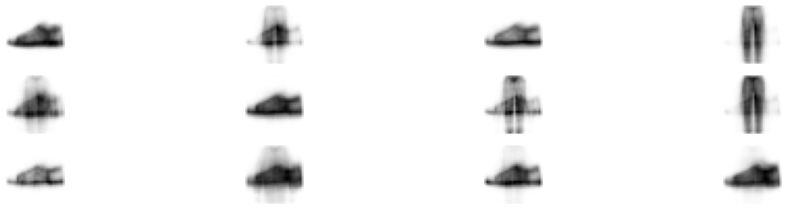
Generate Fashion MNIST image
Use the variational automatic encoder to generate fashionable looking items. All we need to do is sample random codes from Gaussian distribution and decode them
coding = tf.random.normal(shape=[12, codings_size])
images = variational_decoder(coding).numpy()
import matplotlib.pyplot as plt


def plot_image(image):
    plt.imshow(image, cmap='binary')
    plt.axis('off')


fig = plt.figure(figsize=(12 * 1.5, 3))
for image_index in range(12):
    plt.subplot(3, 4, image_index + 1)
    plot_image(images[image_index])
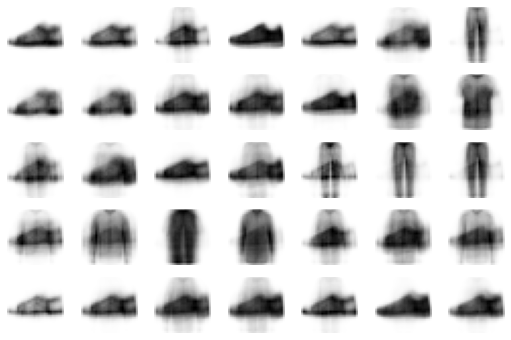
The variable automatic encoder makes semantic interpolation possible: two images can be interpolated at the coding level rather than at the pixel level (it looks like the two images are superimposed). First, let the two images pass through the encoder, then interpolate the obtained two codes, and finally decode the interpolated codes to obtain the final image. It looks like a conventional Fashion MNIST image, but it is an intermediate image between the original images. In the following code example, use the 12 encoders just generated, organize them in the \ (3\times4 \) grid, and then use the TF of TensorFlow image. The resize() function resizes the grid to \ (5\times7 \). By default, the resize() function performs bilinear interpolation, so interpolation codes are included every other row and column. Then, all images are generated using the decoder:
codings_grid = tf.reshape(coding, [1, 3, 4, codings_size])
larger_grid = tf.image.resize(codings_grid, size=[5, 7])
interpolated_codings = tf.reshape(larger_grid, [-1, codings_size])
images = variational_decoder(interpolated_codings).numpy()
fig = plt.figure(figsize=(6 * 1.5, 6))
for image_index in range(35):
    plt.subplot(5, 7, image_index + 1)
    plot_image(images[image_index])