Tips:
① There is no principle here, only R code, running results and interpretation of some results!!!
② There are repetitive parts. If you save time, you can focus on the yellow ones

Case 1 diagnosis of strong influence point

Data description
Regression analysis:

It can be seen from the results that the regression coefficient is not significant and the fitting effect of the model is not good

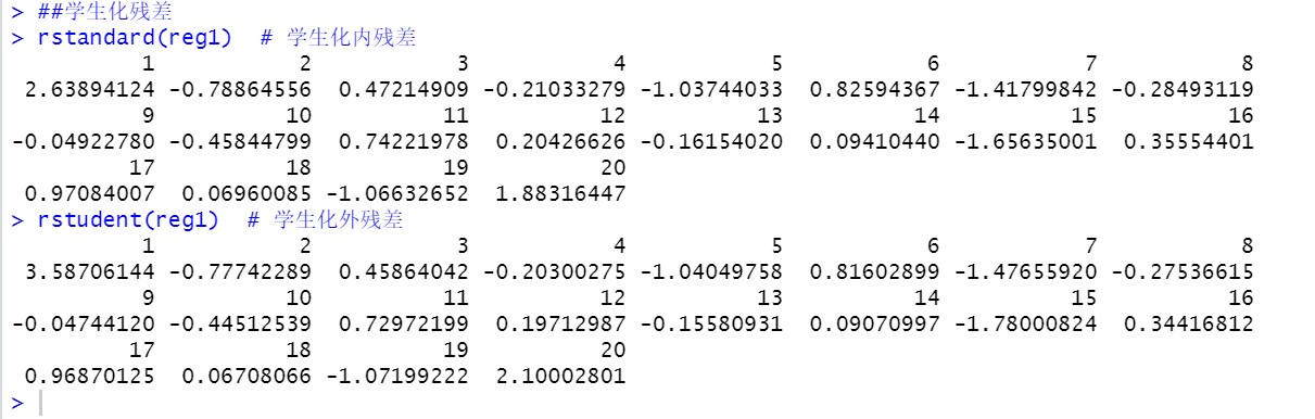
Student residuals:

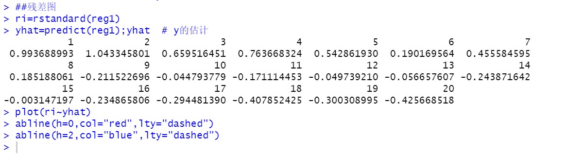
Draw residual diagram:


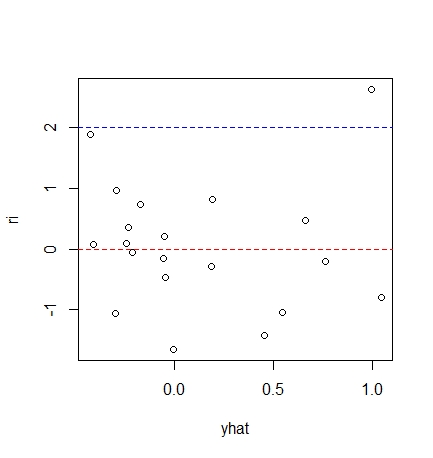
As can be seen from the residual diagram, most of the data are within twice the standard deviation The residual tends to decrease, so the homogeneity assumption of random error term may not be reasonable

Draw regression diagnosis diagram:

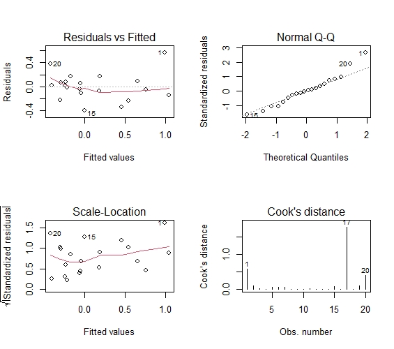
Residuals vs Fitted: the relationship between residuals and estimated values. The data points should be roughly twice the standard deviation, that is, between 2 and - 2, and these points should not show any regular trend
Normal QQ: if the normal hypothesis is satisfied, the point on the graph should fall on a straight line with an angle of 45 degrees; If not, then the assumption of normality is violated
Scale location: the homovariance in GM hypothesis can be diagnosed by this chart, and the variance should be basically determined or flat
Cook's distance: Cook distance, used for diagnosis of strong influence points

Impact analysis:

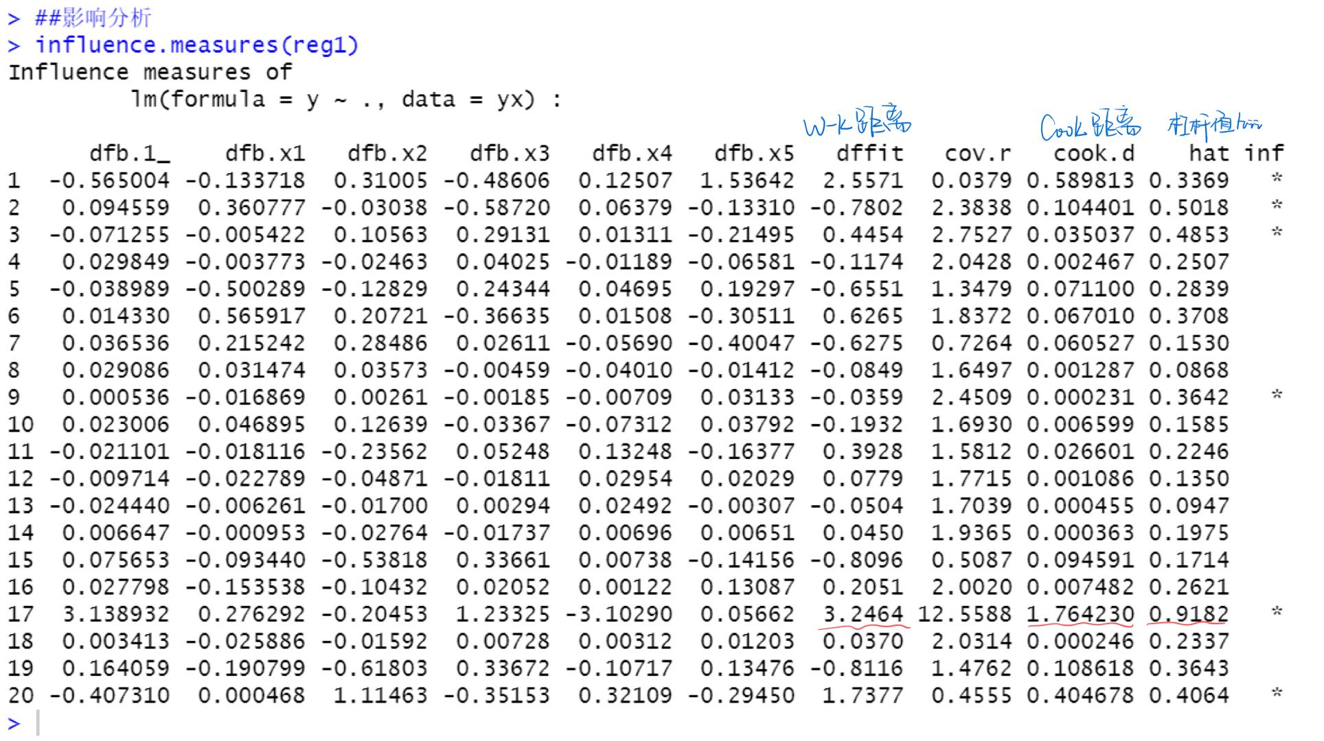
Various impact measures of point 17 are very large, so it is considered that point 17 is a strong impact point Use the influencePlot() function of car package to find out the outliers and strong influence points affecting the regression

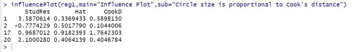
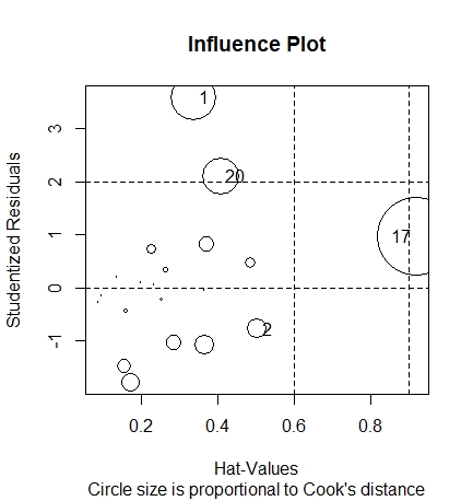
The points with large circles in the figure may be the strong influence points that have a strong influence on the estimation of model parameters

code:

yx=read.table("eg5.6_ch5.txt",header=T)
yx

reg1=lm(y~.,data=yx)
summary(reg1)

sse = 0.2618**2*14
r2 =0.8104
sst = sse/(1-r2)
Ft = 11.97
ssr = sst - sse;ssr
(ssr/5)/(sse/14)

##Studentized residual 
rstandard(reg1)  # Student internal residual
0.562611/(0.2618*sqrt(1-0.3369))
rstudent(reg1)  # Student externalized residual


##Residual diagram
ri=rstandard(reg1)
yhat=predict(reg1);yhat  # Estimation of y
plot(ri~yhat)
abline(h=0,col="red",lty="dashed")
abline(h=2,col="blue",lty="dashed")

##4 residual diagnosis charts
op<-par(mfrow=c(2,2))   # 2 * 2 subgraph
plot(reg1,1:4)
par(op)

##impact analysis 
influence.measures(reg1)

library(car)
influencePlot(reg1,main="Influence Plot",sub="Circle size is proportional to Cook's distance")

Case 2 heteroscedasticity diagnosis

Regression analysis:

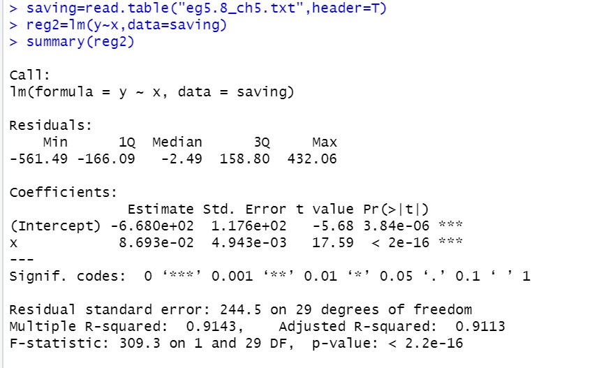
Recall how to read the result

Draw residual diagram:


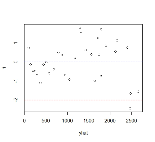
It can be seen from the figure that the points gradually spread from left to right, indicating that the error term has heteroscedasticity

Rank correlation coefficient method to test heteroscedasticity:

        H 0 : r s = 0 H_0:r_s=0 H0: rs = 0 (same variance), H 1 : r s ≠ 0 H_1:r_s\neq0 H1: rs  = 0 (heteroscedasticity) So at the significance level of 0.05, p value 0.001301 < 0.05 0.001301 < 0.05 0.001301 < 0.05, reject the original hypothesis, indicating that the random error term has heteroscedasticity

BP inspection:

p value and significance level α \alpha α The comparison is the same as the rank correlation coefficient method

GQ inspection:

White test:

Heteroscedasticity corrected by weighted least squares:
(anova analysis of variance)

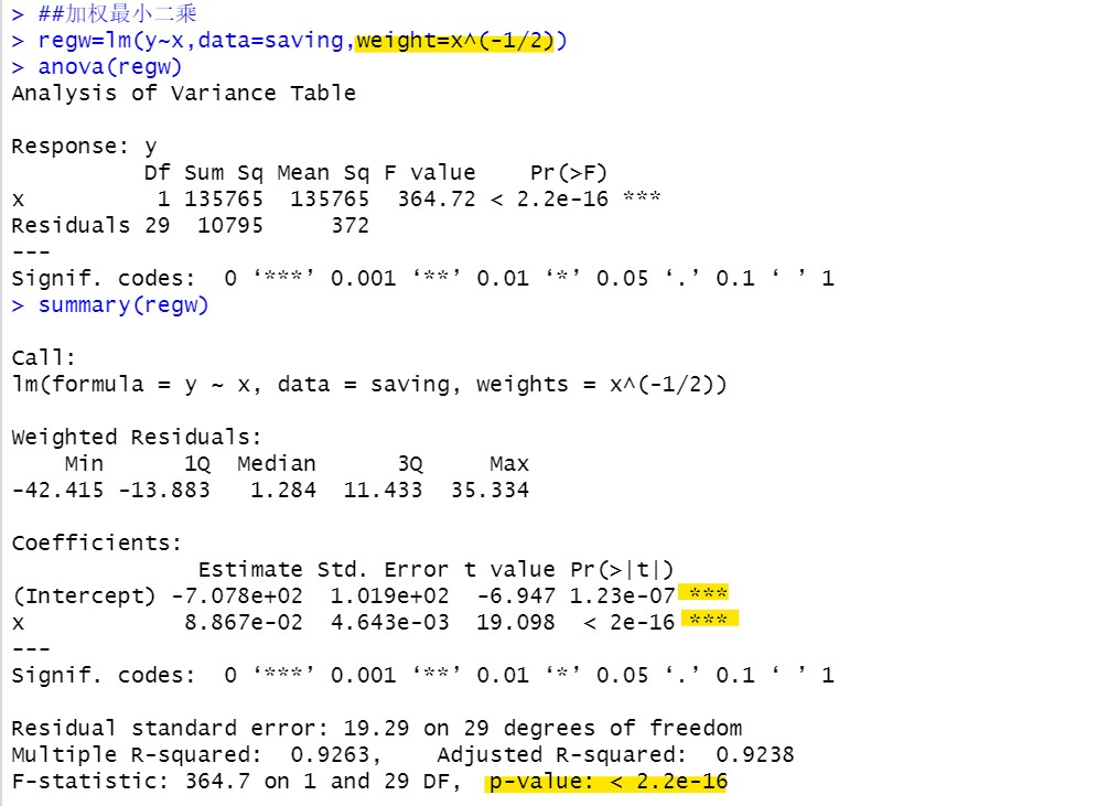
After correcting heteroscedasticity, the results of the model are more accurate

code:

saving=read.table("eg5.8_ch5.txt",header=T)

reg2=lm(y~x,data=saving)
summary(reg2)

plot(y~x,data=saving,col="red")
abline(reg2,col="blue")

##Residual diagram
ri=rstandard(reg2)
yhat=predict(reg2)
plot(ri~yhat)
abline(h=0,col="blue",lty="dashed")
abline(h=-2,col="red",lty="dashed")

##spearman test
abe=abs(reg2$residual)
cor.test(~abe+x,data=saving,method="spearman")

##BP test
#Inspection results
library(lmtest)
library(zoo)
bptest(reg2,studentize=FALSE)
bptest(reg2) #Student orientation can correct heteroscedasticity

#Auxiliary regression results
e=residuals(reg2)
e2=(reg2$residuals)^2;
lmre=lm(e2~saving$x)
summary(lmre)
LM=31*0.2723; LM

##GQ test(lmtest package)
gqtest(reg2)

##white test(whitestrap package)
#Inspection results
# install.packages('whitestrap')
library(whitestrap)
white_test(reg2)

#Auxiliary regression results
x=saving$x
lmre2=lm(e2~x+I(x^2))
summary(lmre2)
white=31*0.2974; white

##Weighted least squares
regw=lm(y~x,data=saving,weight=x^(-1/2))
anova(regw)
summary(regw)

Case 3 autocorrelation diagnosis

(same data as example 2)

DW inspection: remember to see the applicable conditions!!!

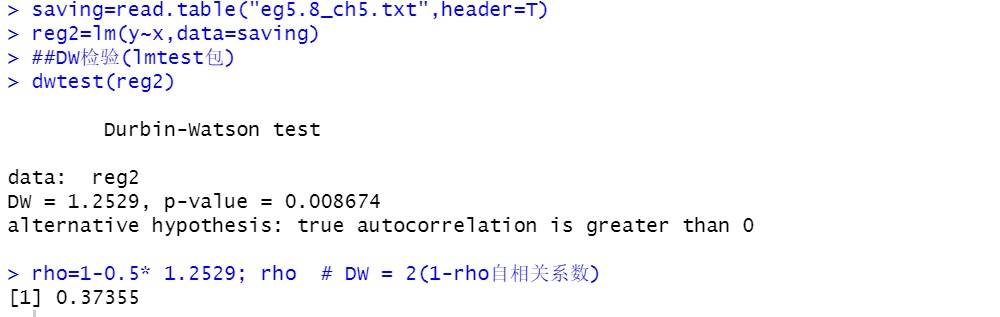
DW=1.2529, R will not directly give the corresponding upper and lower limits, so you need to check the upper and lower limits in the DW distribution table and compare them with DW Or look at p-value, p-value=0.008674 and significance level α \alpha α Comparison, if p < α p<\alpha p< α Reject the original hypothesis and consider that there is first-order autocorrelation
The estimated value of autocorrelation coefficient is 0.37355, indicating that there is moderate autocorrelation in the error term

Lagrange multiplier test: order is the order to be tested

Significance level α = 0.05 \alpha =0.05 α=0.05
o r d e r = 1 order=1 When order=1, p − v a l u e = 0.0546 p-value=0.0546 p − value=0.0546 because p > α p > \alpha p> α， We cannot reject the original hypothesis that there is no significant first-order autocorrelation in this model
o r d e r = 5 order=5 When order=5, p − v a l u e = 0.03772 p-value=0.03772 p − value=0.03772 because p < α p < \alpha p< α， Rejecting the original hypothesis, it is considered that there is a significant fifth order autocorrelation in this model

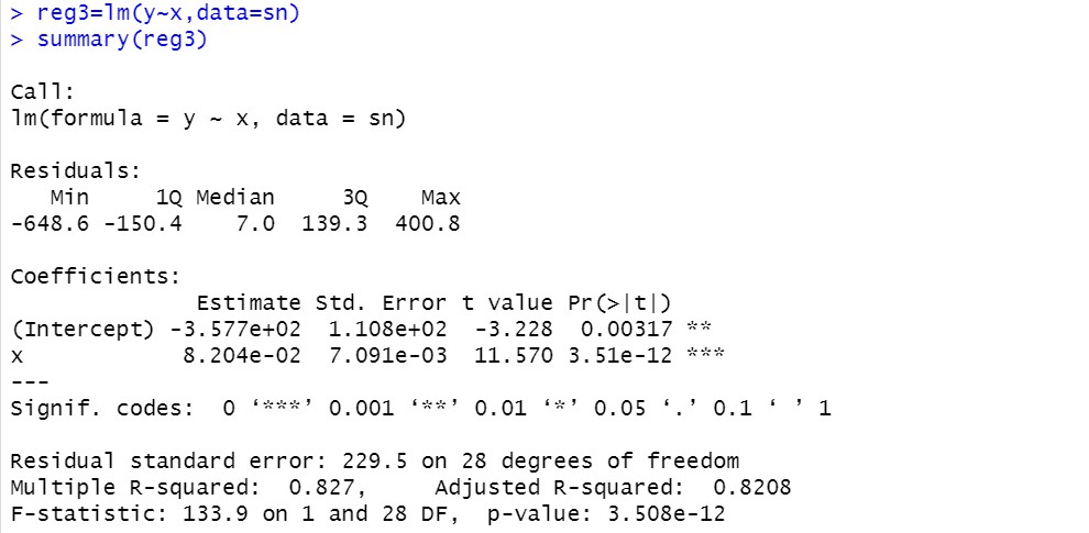
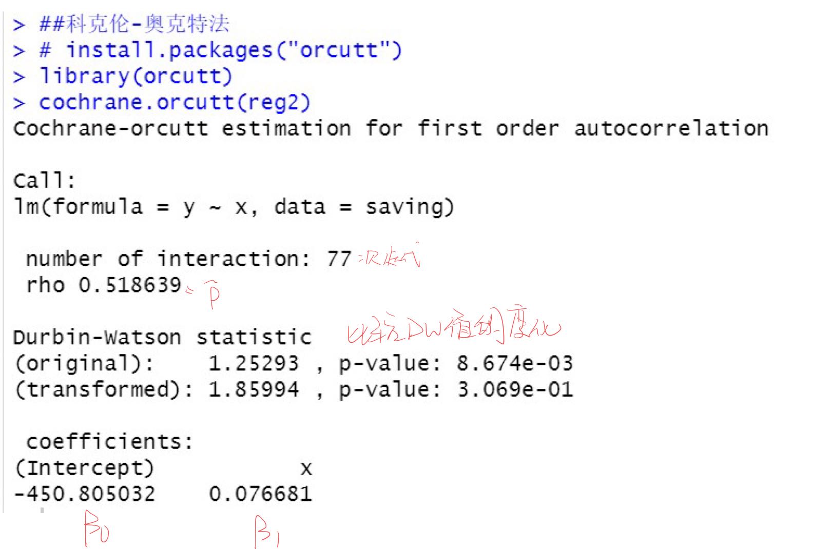
Elimination of autocorrelation by generalized difference method: only applicable to first-order autocorrelation

Elimination of autocorrelation by Cochran oakt iterative method: it is only applicable to high-order autocorrelation of second-order and above

code:

saving=read.table("eg5.8_ch5.txt",header=T)
reg2=lm(y~x,data=saving)

##DW inspection (lmtest package)
dwtest(reg2)
rho=1-0.5* 1.2529; rho  # DW = 2(1-rho autocorrelation coefficient)

##lagrange multiplier test 
bgtest(reg2,order=1)
bgtest(reg2,order=5)

##Generalized difference
n=nrow(saving)
st=saving[-1,]
stlag1=saving[1:(n-1),]
sn=st-rho*stlag1  # DW
cbind(st,stlag1,sn)  # Two or three columns lag one period, and the last two columns of generalized difference
reg3=lm(y~x,data=sn)
summary(reg3)

##Cochran oakt method
# install.packages("orcutt")
library(orcutt)
cochrane.orcutt(reg2)

Case 4 multiple collinearity diagnosis

Visual diagnosis of correlation coefficient matrix:

From the correlation coefficient matrix, we can see that there are at least two groups of significant negative linear correlations in the explanatory variables
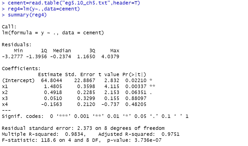
Regression diagnosis:

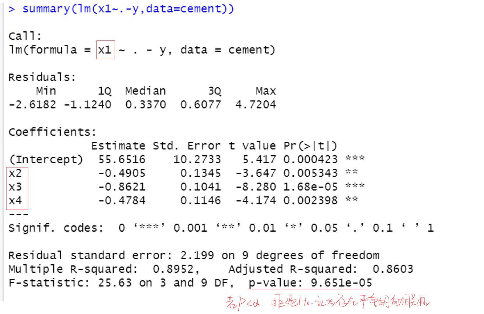
It's only done here x 1 x_1 x1 auxiliary regression equation with other explanatory variables, others can try by yourself

Variance inflation factor diagnosis:

Judgment method 1: if the variance expansion factor is greater than 10, it is considered that there is serious multicollinearity Therefore, the above results show that there are two groups of serious multicollinearity
Judgment method 2: if the average value of the four VIFS is greater than 1, it indicates that there is serious multicollinearity

Diagnostic method of characteristic root and condition number:

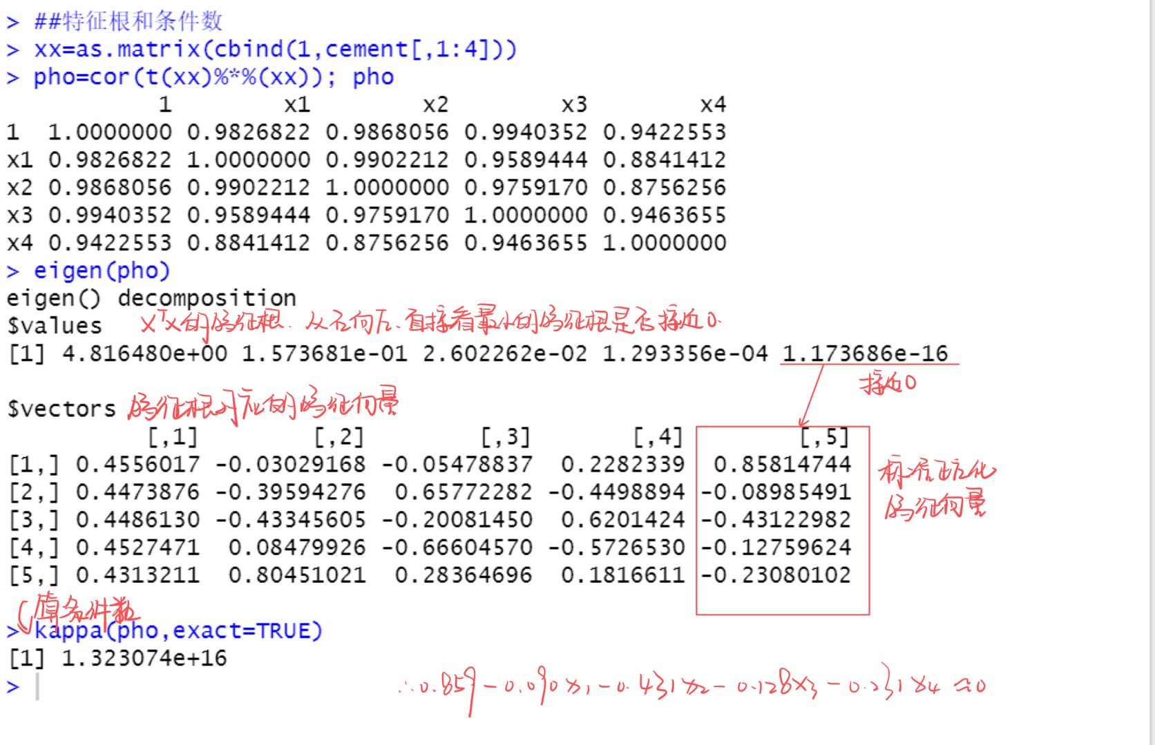
When at least one eigenvalue is approximately 0, there must be multicollinearity between explanatory variables
Severe multicollinearity is considered when the condition number is greater than 100

code:

cement=read.table("eg5.10_ch5.txt",header=T)
reg4=lm(y~.,data=cement)
summary(reg4)

cor(cement)
summary(lm(x1~.-y,data=cement))

##VIF
# install.packages('DAAG')
library(DAAG)
vif(reg4,digit=3)


##Characteristic root and condition number
xx=as.matrix(cbind(1,cement[,1:4]))
pho=cor(t(xx)%*%(xx)); pho
eigen(pho)
kappa(pho,exact=TRUE)