Original link: http://tecdat.cn/?p=20650

People usually use receiver operating characteristic curve (ROC) for binary result logistic regression. However, the outcome of interest in epidemiological studies is usually the time of the event. The prediction model in this case can be described more comprehensively by using the time-dependent ROC varying with time.

Time dependent ROC definition

Let Mi be the baseline (time 0) scalar marker for mortality prediction. When results are observed over time, their predictive performance depends on the evaluation time_ t_. Intuitively, the marker values measured at zero time should become less relevant. Therefore, the predicted performance (discrimination) measured by ROC is time_ t_ Function of.

Cumulative cases

Cumulative case / dynamic ROC defined in time_ t_ Threshold at_ c_ The sensitivity and specificity are as follows.

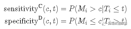
The cumulative sensitivity will change over time_ t_ Those who died before are regarded as the denominator (disease), and the marker value is higher than_ c_ As a real positive disease. Dynamic specificity will be in time_ t_ Still alive as the denominator (healthy) and mark the value less than or equal to_ c_ Those are considered true negatives (negatives in health). Set threshold_ c_ Changing from the minimum to the maximum will occur in time_ t_ The entire ROC curve is displayed at.

New cases

When is the new case ROC1_ t_ At threshold_ c_ Sensitivity and specificity are defined as follows.

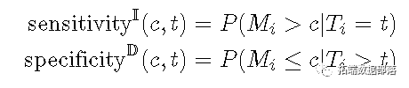
The cumulative sensitivity will change over time_ t place_ The dead person is regarded as the denominator (disease), and the marker value is higher than_ Ç_ People are considered true positive (disease positive).

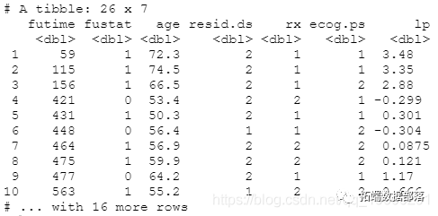
Data preparation

Let's take ovarian dataset3 survival in the packet as an example. The time of the event is the time of death. The Kaplan Meier diagram is as follows.

 ## Become data_frame
data <- as_data_frame(data)
## mapping
plot(survfit(Surv(futime, fustat) ~ 1,
                   data = data)

Visualization results:

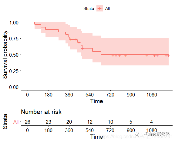
No events occurred in the dataset for more than 720 days.

 ## Fitting cox model
coxph(formula = Surv(futime, fustat) ~ pspline(age, df = 4) + 
##Obtain linear prediction value
 predict(coxph1, type = "lp")

Cumulative cases

Cumulative cases were achieved

 ## Define an auxiliary function to evaluate at different times
ROC_hlp <- function(t) {
    survivalROC(Stime        
                status        
                marker        
                predict.time = t,
                method       = "NNE",
                span = 0.25 * nrow(ovarian)^(-0.20))
}
## Evaluate every 180 days
ROC_data <- data_frame(t = 180 * c(1,2,3,4,5,6)) %>%
    mutate(survivalROC = map(t, survivalROC_helper),
           ## Extract AUC
           auc = map_dbl(survivalROC, magrittr::extract2, "AUC"),
           ## In data_ Put relevant values in frame
           df_survivalROC = map(survivalROC, function(obj) {
           
## mapping
 ggplot(mapping = aes(x = FP, y = TP)) +
    geom_point() +
    geom_line() +
      facet_wrap( ~ t) +

Visualization results:

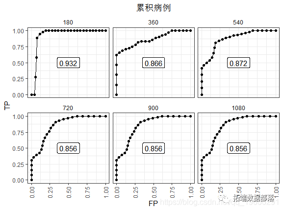
The 180 day ROC looks the best. Because there have been few events so far. After the last observed event (t ≥ 720), the AUC stabilized at 0.856. This performance did not decline because people with high risk scores died.

New cases

Achieve new cases

 ## Define an auxiliary function to evaluate at different times
 
## Evaluate every 180 days
 
            ## Extract AUC
           auc = map_dbl(risksetROC, magrittr::extract2, "AUC"),
           ## In data_ Put relevant values in frame
           df_risksetROC = map(risksetROC, function(obj) {
               ## Marker bar
               marker <- c(-Inf, obj[["marker"]], Inf)
 
## mapping
 
    ggplot(mapping = aes(x = FP, y = TP)) +
    geom_point() +
    geom_line() +
    geom_label(data = risksetROC_data %>% dplyr::select(t,auc) %>% unique,
    facet_wrap( ~ t) +

Visualization results:

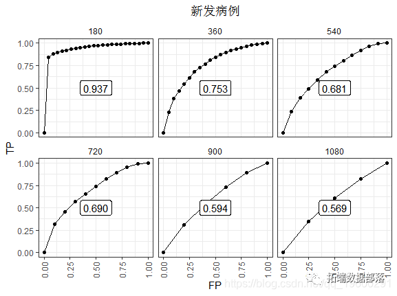
This difference is more obvious in the later stage. Most notably, only individuals at risk concentration at each point in time can provide data. So there are fewer data points. The decline in performance is more obvious, perhaps because the risk score of time zero is less important in those who survive long enough. Once there are no events, the ROC will basically flatten.

conclusion

In conclusion, we study the time-dependent ROC and its R implementation. Cumulative case ROC may be related to_ Risk_ The concept of (cumulative incidence) prediction model is more compatible. The ROC of new cases can be used to examine the correlation of time zero markers in predicting subsequent events.

reference resources

1. Heagerty,Patrick J. and Zheng,Yingye, _Survival Model Predictive Accuracy and ROC Curves_,Biometrics，61(1),92-105(2005). doi: 10.1111 / j.0006-341X.2005.030814.x.

This paper is an excerpt from visualization of time-dependent ROC curve of survival analysis model in R language