1. Introduction of GloVe word vector

GloVe: The full name is Global Vectors for Word Representations. Its document [2] was presented at the EMNLP conference in 2014. It combines the idea of word vector and matrix decomposition to pre-train the original corpus and get a low-dimensional, continuous and sparse representation. Visualizing the pre-trained word vector can discover the relationship between some words.
(Appendix: 2 commonly used methods for estimating word vectors,
1 is a language model based on neural network and word vector pre-training method based on word2vec, which essentially uses the co-occurrence information of words and words in local context as self-supervised learning signals.
2. Matrix-based decomposition methods, such as LSA (Latent Semantic Analysis Latent Semantic Semantic Analysis), start with statistical analysis of the corpus, obtain a word-context co-occurrence matrix with global statistical information, and then use Singular Value Decomposition (SVD)However, the word vector obtained by the traditional matrix decomposition method does not have good geometric properties, so the GloVe word vector is proposed, which combines the word vector with the idea of matrix decomposition and has a better result. [1]

2. Introduction to t-SNE

t-SNE, full name t-distributed stochastic neighbor embedding. I don't know much about the process, but it can compress high-dimensional data into low-dimensional output.
If the input is (n_sample, n_dimension), the output is (n_sample, 2). This process compresses samples with n_sample dimensions into two dimensions.

3. Pre-trained GloVe word vectors

Pre-trained word vectors are placed on the official website, please download them yourself:
(Web address:https://nlp.stanford.edu/projects/glove/)

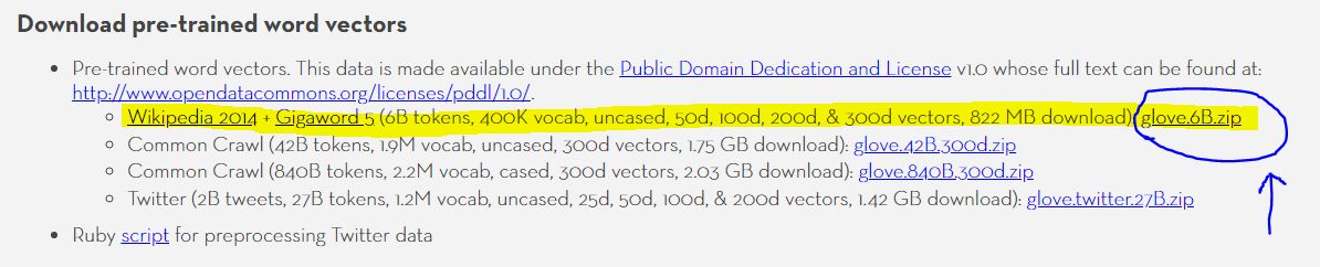
As shown in the figure above, there are different pre-training models based on different corpuses, such as corpus information crawled from Wikipedia, Twitter, and normal. I chose the first one, which is the data crawled from Wikipedia.
After unzipping the file, glove.6B.50d.txt was selected (that is, 400 K vocabs were extracted from 6B token s, each with a 50-dimensional vocab).
Looking at any five lines extracted from the txt document, we find that the first number of each line is token, and the remaining 50 float-type numbers are the 50-dimensional representation of the token.

were 0.73363 -0.74815 0.45913 -0.56041 0.091855 0.33015 -1.2034 -0.15565 -1.1205 -0.5938 0.23299 -0.46278 -0.34786 -0.47901 0.57621 -0.16053 -0.26457 -0.13732 -0.91878 -0.65339 0.05884 0.61553 1.2607 -0.39821 -0.26056 -1.0127 -0.38517 -0.096929 -0.11701 -0.48536 3.6902 0.30744 0.50713 -0.6537 0.80491 0.23672 0.61769 0.030195 -0.57645 0.60467 -0.63949 -0.11373 0.84984 0.41409 0.083774 -0.28737 -1.4735 -0.20095 -0.17246 -1.0984
not 0.55025 -0.24942 -0.0009386 -0.264 0.5932 0.2795 -0.25666 0.093076 -0.36288 0.090776 0.28409 0.71337 -0.4751 -0.24413 0.88424 0.89109 0.43009 -0.2733 0.11276 -0.81665 -0.41272 0.17754 0.61942 0.10466 0.33327 -2.3125 -0.52371 -0.021898 0.53801 -0.50615 3.8683 0.16642 -0.71981 -0.74728 0.11631 -0.37585 0.5552 0.12675 -0.22642 -0.10175 -0.35455 0.12348 0.16532 0.7042 -0.080231 -0.068406 -0.67626 0.33763 0.050139 0.33465
this 0.53074 0.40117 -0.40785 0.15444 0.47782 0.20754 -0.26951 -0.34023 -0.10879 0.10563 -0.10289 0.10849 -0.49681 -0.25128 0.84025 0.38949 0.32284 -0.22797 -0.44342 -0.31649 -0.12406 -0.2817 0.19467 0.055513 0.56705 -1.7419 -0.91145 0.27036 0.41927 0.020279 4.0405 -0.24943 -0.20416 -0.62762 -0.054783 -0.26883 0.18444 0.18204 -0.23536 -0.16155 -0.27655 0.035506 -0.38211 -0.00075134 -0.24822 0.28164 0.12819 0.28762 0.1444 0.23611
who -0.19461 -0.051277 0.26445 -0.57399 1.0236 0.58923 -1.3399 0.31032 -0.89433 -0.13192 0.21305 0.29171 -0.66079 0.084125 0.76578 -0.42393 0.32445 0.13603 -0.29987 -0.046415 -0.74811 1.2134 0.24988 0.22846 0.23546 -2.6054 0.12491 -0.94028 -0.58308 -0.32325 2.8419 0.33474 -0.33902 -0.23434 0.37735 0.093804 -0.25969 0.68889 0.37689 -0.2186 -0.24244 1.0029 0.18607 0.27486 0.48089 -0.43533 -1.1012 -0.67103 -0.21652 -0.025891
they 0.70835 -0.57361 0.15375 -0.63335 0.46879 -0.066566 -0.86826 0.35967 -0.64786 -0.22525 0.09752 0.27732 -0.35176 -0.25955 0.62368 0.60824 0.34905 -0.27195 -0.27981 -1.0183 -0.1487 0.41932 1.0342 0.17783 0.13569 -1.9999 -0.56163 0.004018 0.60839 -1.0031 3.9546 0.68698 -0.53593 -0.7427 0.18078 0.034527 0.016026 0.12467 -0.084633 -0.10375 -0.47862 -0.22314 0.25487 0.69985 0.32714 -0.15726 -0.6202 -0.23113 -0.31217 -0.3049

4.Programming uses t-SNE to visualize Glove vectors.

The scikit-learn s library contains the implementation of t-SNE. Combined with the code given by the authorities, the Glove word vector for t-SNE visualization is implemented here. In addition, only the first 100 Glove vectors are shown here due to the clutter and arithmetic limitations of the picture when there are too many tokens. Interested readers can also extract specific tokens and different number of tokens from this code for visualization.

The code is as follows:

import numpy as np
import matplotlib.pyplot as plt
from matplotlib import offsetbox
from sklearn.preprocessing import MinMaxScaler
from sklearn.manifold import TSNE
from time import time
from sklearn.datasets import load_digits

digits = load_digits(n_class=6)

# 1. Read the GloVe vector database in 6 categories. There are 400,000 token s, each of which is 50 dimensions.
glove_txt = "/home/lwq/20210922/glove.6B.50d.txt"
with open(glove_txt) as f:
    lines = f.readlines()
    lines = lines[:100]
    X = []
    y = []
    for line in lines:
        now = line.split(' ')
        y.append(now[0])
        X.append(now[1:])
    X = np.array(X)
    y = np.array(y)

n_samples, n_features = X.shape


# 2. Write drawing functions to draw the input data X.
def plot_embedding(X, title, ax):
    X = MinMaxScaler().fit_transform(X)

    shown_images = np.array([[1.0, 1.0]])  # just something big
    for i in range(X.shape[0]):
        # plot every digit on the embedding
        ax.text(
            X[i, 0],
            X[i, 1],
            str(y[i]),
            # color=plt.cm.Dark2(y[i]),
            fontdict={"weight": "bold", "size": 9},
        )
        '''
        # show an annotation box for a group of digits
        dist = np.sum((X[i] - shown_images) ** 2, 1)
        if np.min(dist) < 4e-3:
            # don't show points that are too close
            continue
        shown_images = np.concatenate([shown_images, [X[i]]], axis=0)
        imagebox = offsetbox.AnnotationBbox(
            offsetbox.OffsetImage(digits.images[i], cmap=plt.cm.gray_r), X[i]
        )
        ax.add_artist(imagebox)
        '''
    ax.set_title(title)
    ax.axis("off")


# 3. Choose which way you want to encode the raw data (Embedding), and choose TSNE here.
#  n_components = 2 means the output is 2-dimensional, learning_rate defaults to 200.0,
embeddings = {
    "t-SNE embeedding": TSNE(
        n_components=2, init='pca', learning_rate=200.0, random_state=0
    ),
}


# 4. Generate a compressed encoding matrix based on the encoding method in the dictionary (TSNE only here)
# That is, each sample is represented in two dimensions. The dimensions change from 50 to 2.
# Input: (n_sample, n_dimension)
# Output: (n_sample, 2)

projections, timing = {}, {}
for name, transformer in embeddings.items():
    # Of the original author dict There are many ways to compare, I only use t-SNE,You can query the original link if you want: https://scikit-learn.org/stable/auto_examples/manifold/plot_lle_digits.html#manifold-learning-on-handwritten-digits-locally-linear-embedding-isomap
    if name.startswith("Linear Discriminant Analysis"):
        data = X.copy()
        data.flat[:: X.shape[1] + 1] += 0.01  # Make X invertible
    else:
        data = X

    print(f"Computing {name}...")
    start_time = time()
    print(data.shape, type(data.shape))
    projections[name] = transformer.fit_transform(data, y)
    timing[name] = time() - start_time



# 6. Output the encoding matrix into a two-dimensional image.
fig, ax = plt.subplots()
title = f"{name} (time {timing[name]:.3f}s)"
plot_embedding(projections[name], title, ax)
plt.show()

The results are as follows:

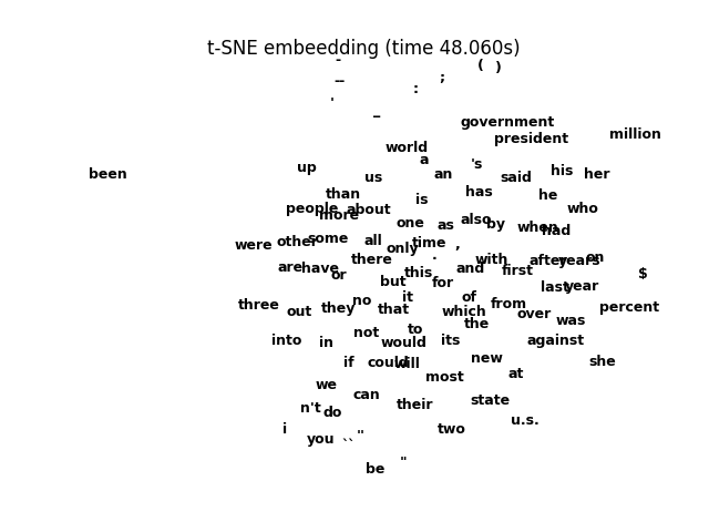
Image above: Visualize the first 100 GloVe word vectors using t-SNE

From the diagram, we can see that the top punctuation symbols are grouped together to show that they are similar. his, her, he, who are grouped together. year and years are grouped together to show some semantic similarity. This may show different results on different corpus and different dimensions.

The results show that the Glove word vector has some correlation. However, the GloVe word vector is a static word vector and cannot solve the problem of "word ambiguity" in NLP tasks. Therefore, some dynamic word vector representations, such as Elmo model, and pretraining models such as GPT and BERT, which are now especially popular, can be considered.

Reference

1. Natural Language Processing: Method Based on Pre-training Model. Che Wanxiang et al., 2021.
2.Jeffrey Pennington, Richard Socher, and Christopher D. Manning. 2014. GloVe: Global Vectors for Word Representation.
3.https://scikit-learn.org/stable/auto_examples/manifold/plot_lle_digits.html#manifold-learning-on-handwritten-digits-locally-linear-embedding-isomap