abstract
In order to understand what happened, we printed out some statistics during model training to see whether the training was in progress. However, we can do better: PyTorch is integrated with TensorBoard, which is a tool for visualizing the results of neural network training. This tutorial explains some of its functions using the fashion MNIST dataset, which can be read into PyTorch using torchvision.datasets.
In this tutorial, we will learn how to:
- Read in the data and make the appropriate transformation (almost the same as the previous tutorial).
- Set TensorBoard.
- Write to TensorBoard.
- Use TensorBoard to check the model schema.
- Use TensorBoard to create an interactive version of the visualization we created in the previous tutorial with less code
Specifically, in point 5, we will see how several methods to check the training data track the performance of the model during training and evaluate the performance of the model after training.
We'll start with template code similar to that in the CIFAR-10 tutorial:
# imports
import matplotlib.pyplot as plt
import numpy as np

import torch
import torchvision
import torchvision.transforms as transforms

import torch.nn as nn
import torch.nn.functional as F
import torch.optim as optim

# transforms
transform = transforms.Compose(
    [transforms.ToTensor(),
    transforms.Normalize((0.5,), (0.5,))])

# datasets
trainset = torchvision.datasets.FashionMNIST('./data',
    download=True,
    train=True,
    transform=transform)
testset = torchvision.datasets.FashionMNIST('./data',
    download=True,
    train=False,
    transform=transform)

# dataloaders
trainloader = torch.utils.data.DataLoader(trainset, batch_size=4,
                                        shuffle=True, num_workers=2)


testloader = torch.utils.data.DataLoader(testset, batch_size=4,
                                        shuffle=False, num_workers=2)

# constant for classes
classes = ('T-shirt/top', 'Trouser', 'Pullover', 'Dress', 'Coat',
        'Sandal', 'Shirt', 'Sneaker', 'Bag', 'Ankle Boot')

# helper function to show an image
# (used in the `plot_classes_preds` function below)
def matplotlib_imshow(img, one_channel=False):
    if one_channel:
        img = img.mean(dim=0)
    img = img / 2 + 0.5     # unnormalize
    npimg = img.numpy()
    if one_channel:
        plt.imshow(npimg, cmap="Greys")
    else:
        plt.imshow(np.transpose(npimg, (1, 2, 0)))
We will define a similar model architecture in this tutorial, with only minor modifications to take into account the fact that the image is now one channel instead of three channels and 28x28 instead of 32x32:
class Net(nn.Module):
    def __init__(self):
        super(Net, self).__init__()
        self.conv1 = nn.Conv2d(1, 6, 5)
        self.pool = nn.MaxPool2d(2, 2)
        self.conv2 = nn.Conv2d(6, 16, 5)
        self.fc1 = nn.Linear(16 * 4 * 4, 120)
        self.fc2 = nn.Linear(120, 84)
        self.fc3 = nn.Linear(84, 10)

    def forward(self, x):
        x = self.pool(F.relu(self.conv1(x)))
        x = self.pool(F.relu(self.conv2(x)))
        x = x.view(-1, 16 * 4 * 4)
        x = F.relu(self.fc1(x))
        x = F.relu(self.fc2(x))
        x = self.fc3(x)
        return x


net = Net()
We will define the same optimizer and standard as before:
criterion = nn.CrossEntropyLoss()
optimizer = optim.SGD(net.parameters(), lr=0.001, momentum=0.9)
1. TensorBoard settings
Now we will set up TensorBoard, import TensorBoard from torch.utils and define a SummaryWriter, which is the key object for us to write information to TensorBoard.
from torch.utils.tensorboard import SummaryWriter  #
default `log_dir` is "runs" - we'll be more specific here
writer = SummaryWriter('runs/fashion_mnist_experiment_1')
Note that only this row creates a running/fashion_mnist_experiment_1 folder.
2. Write TensorBoard
Now let's use make_grid writes images to TensorBoard - especially the grid.
# get some random training images
dataiter = iter(trainloader)
images, labels = dataiter.next()

# create grid of images
img_grid = torchvision.utils.make_grid(images)

# show images
matplotlib_imshow(img_grid, one_channel=True)

# write to tensorboard
writer.add_image('four_fashion_mnist_images', img_grid)
Running
3. Use TensorBoard to check the model
One of the advantages of TensorBoard is its ability to visualize complex model structures. Let's visualize the model we build.
writer.add_graph(net, images)
writer.close()
Now after refreshing TensorBoard, you should see a "Graphs" tab as follows:
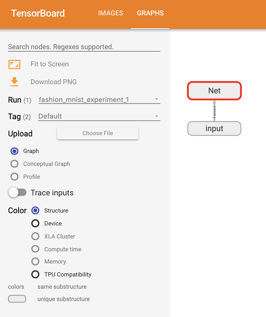
Continue and double-click Net to see its expansion and see a detailed view of the various operations that make up the model.
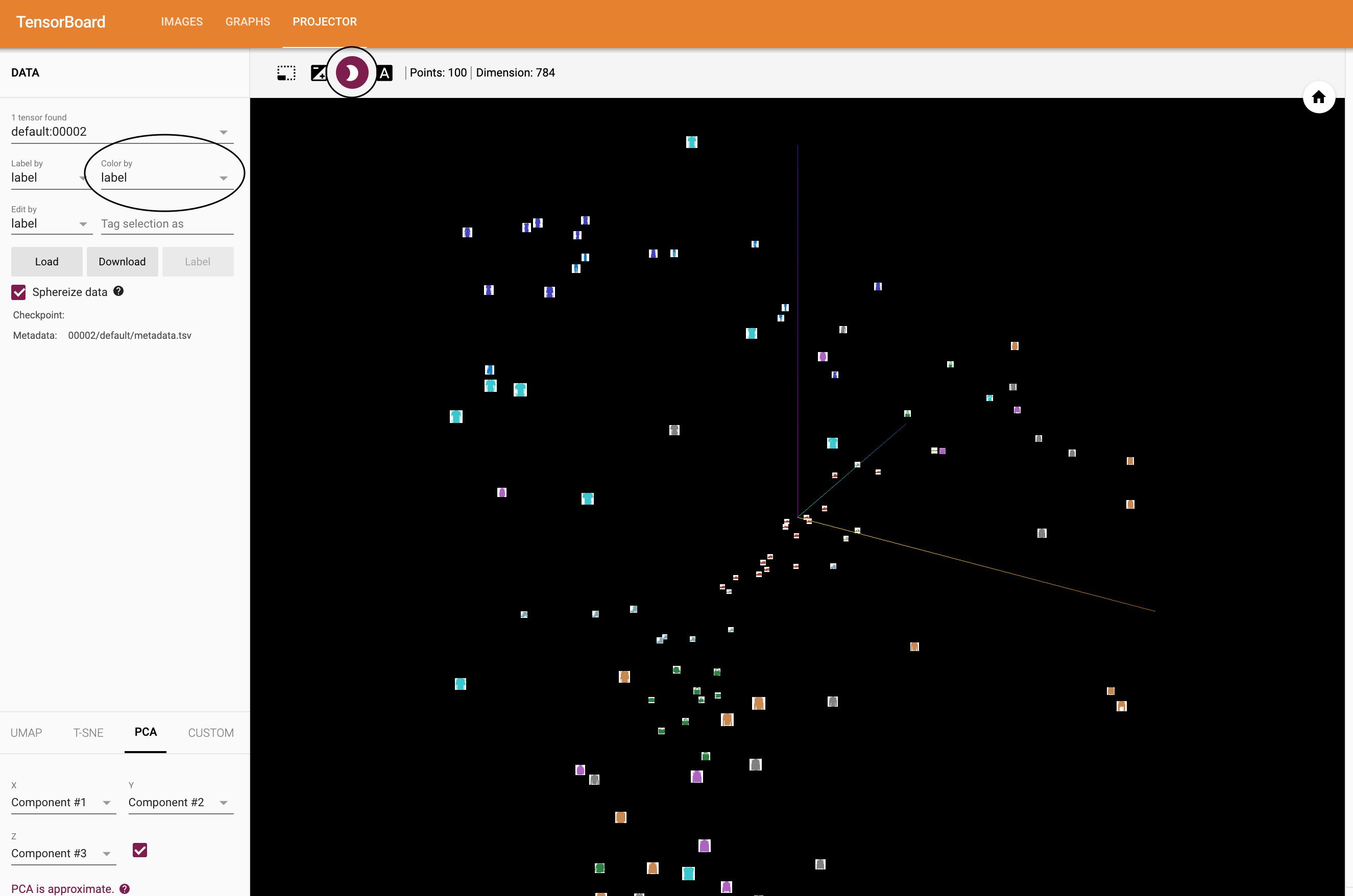
TensorBoard has a very convenient function, which can visualize high-dimensional data in low-dimensional space, such as image data; We'll introduce this next.
4. Add "projector" to TensorBoard
We can add_embedding method for visualizing low dimensional representation of high dimensional data
# helper function
def select_n_random(data, labels, n=100):
    '''
    Selects n random datapoints and their corresponding labels from a dataset
    '''
    assert len(data) == len(labels)

    perm = torch.randperm(len(data))
    return data[perm][:n], labels[perm][:n]

# select random images and their target indices
images, labels = select_n_random(trainset.data, trainset.targets)

# get the class labels for each image
class_labels = [classes[lab] for lab in labels]

# log embeddings
features = images.view(-1, 28 * 28)
writer.add_embedding(features,
                    metadata=class_labels,
                    label_img=images.unsqueeze(1))
writer.close()
Now, in the projector tab of TensorBoard, you can see that these 100 images -- each 784 dimensional -- are projected into 3-dimensional space. In addition, this is interactive: you can click and drag to rotate the 3D projection. Finally, some tips to make visualization easier to see: select the "color: label" in the upper left corner and turn on "night mode", which will make images easier to see because their background is white:
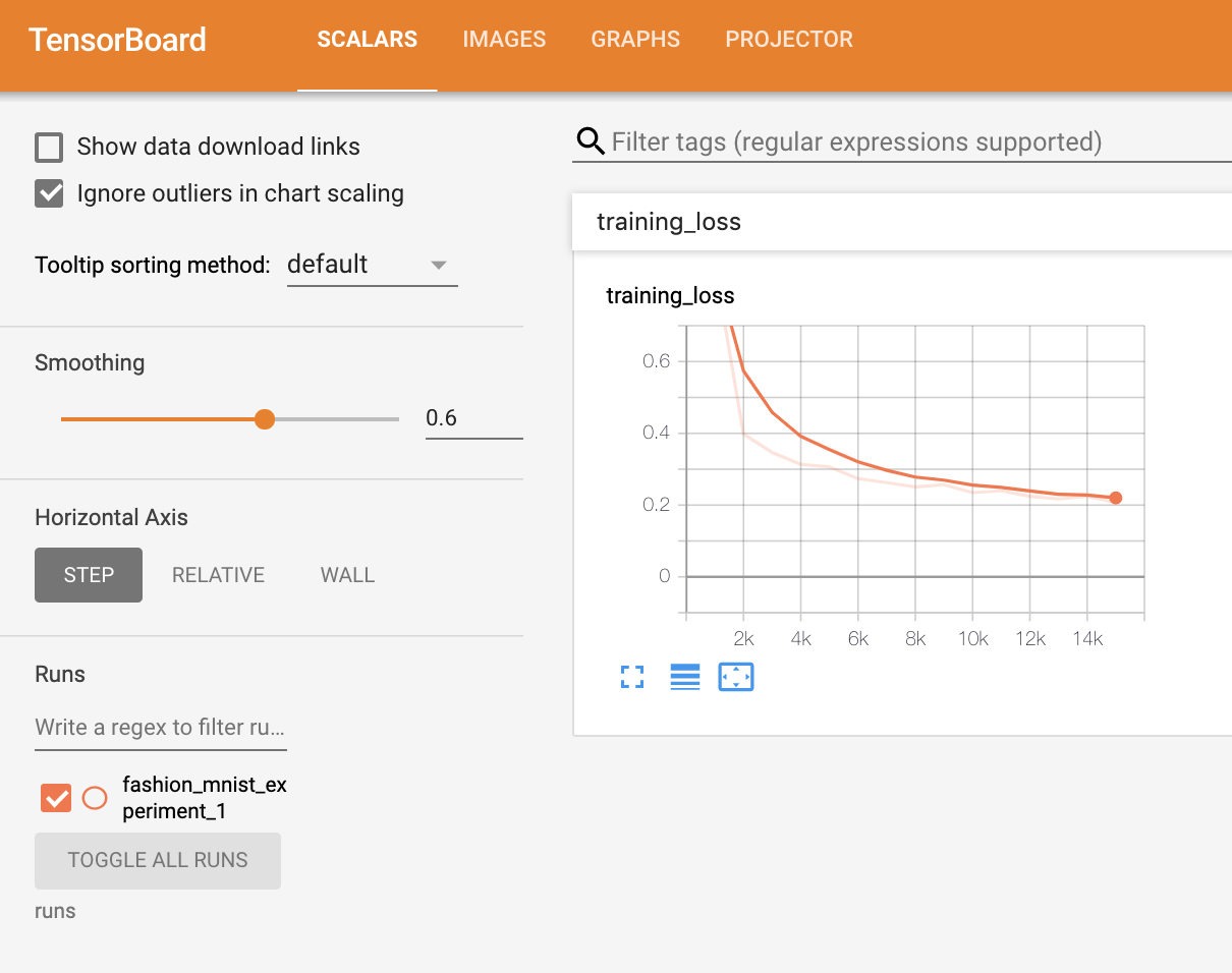
5. Training with TensorBoard tracking model
In the previous example, we simply print the running loss of the model every 2000 iterations. Now, we will record the running loss to TensorBoard and view the model through plot_ classes_ The prediction made by the preds function.
# helper functions

def images_to_probs(net, images):
    '''
    Generates predictions and corresponding probabilities from a trained
    network and a list of images
    '''
    output = net(images)
    # convert output probabilities to predicted class
    _, preds_tensor = torch.max(output, 1)
    preds = np.squeeze(preds_tensor.numpy())
    return preds, [F.softmax(el, dim=0)[i].item() for i, el in zip(preds, output)]


def plot_classes_preds(net, images, labels):
    '''
    Generates matplotlib Figure using a trained network, along with images
    and labels from a batch, that shows the network's top prediction along
    with its probability, alongside the actual label, coloring this
    information based on whether the prediction was correct or not.
    Uses the "images_to_probs" function.
    '''
    preds, probs = images_to_probs(net, images)
    # plot the images in the batch, along with predicted and true labels
    fig = plt.figure(figsize=(12, 48))
    for idx in np.arange(4):
        ax = fig.add_subplot(1, 4, idx+1, xticks=[], yticks=[])
        matplotlib_imshow(images[idx], one_channel=True)
        ax.set_title("{0}, {1:.1f}%\n(label: {2})".format(
            classes[preds[idx]],
            probs[idx] * 100.0,
            classes[labels[idx]]),
                    color=("green" if preds[idx]==labels[idx].item() else "red"))
    return fig
Finally, let's use the same model training code as in the previous tutorial to train the model, but write the results to TensorBoard every 1000 batches instead of printing to the console; This is using add_scalar function.
In addition, during training, we will generate an image to show the prediction of the model and the actual results of the four images contained in the batch.
running_loss = 0.0
for epoch in range(1):  # loop over the dataset multiple times

    for i, data in enumerate(trainloader, 0):

        # get the inputs; data is a list of [inputs, labels]
        inputs, labels = data

        # zero the parameter gradients
        optimizer.zero_grad()

        # forward + backward + optimize
        outputs = net(inputs)
        loss = criterion(outputs, labels)
        loss.backward()
        optimizer.step()

        running_loss += loss.item()
        if i % 1000 == 999:    # every 1000 mini-batches...

            # ...log the running loss
            writer.add_scalar('training loss',
                            running_loss / 1000,
                            epoch * len(trainloader) + i)

            # ...log a Matplotlib Figure showing the model's predictions on a
            # random mini-batch
            writer.add_figure('predictions vs. actuals',
                            plot_classes_preds(net, inputs, labels),
                            global_step=epoch * len(trainloader) + i)
            running_loss = 0.0
print('Finished Training')
You can now view the scalar tab to see the running losses plotted over 15000 training iterations: