ID3 Decision Tree Algorithm
1. Theory
-
purity
For a branch node, if all the samples it contains belong to the same class, its purity is 1, and we always want the higher the purity, the better, that is, as many samples as possible belong to the same class. So how do you measure "purity"? The concept of "information entropy" is introduced. -
information entropy
Assuming that the proportion of class k samples in the current sample set D is pk (k=1,2,..., |y|), the information entropy of D is defined as:Ent(D) = -∑k=1 pk·log2 pk (If agreed p=0,be log2 p=0)
Obviously, the smaller the Ent(D) value, the higher the purity of D. Because 0<=pk<= 1, log2 pk<=0, Ent(D)>=0. In the limit case, if the samples in D belong to the same class, the Ent(D) value is 0 (to the minimum). Ent(D) takes the maximum log2 |y | when the samples in D belong to different categories.
-
information gain
Assume that discrete attribute a has all V possible values {a1,a2,..., av}. If A is used to classify the sample set D, then V branch nodes will be generated. Note that D V is a sample with a V values on all attribute a contained in the V branch node. Different branch nodes have different samples, so we give different weights to the branch nodes: |Dv|/|D|, which gives more influence to the branch nodes with more samples. Therefore, the information gain obtained by dividing the sample set D with attribute a is defined as:Gain(D,a) = Ent(D)-∑v=1 |Dv|/|D|·Ent(Dv)
Ent(D) is the information entropy before the partition of dataset D. _v=1 |D v|/|D|Ent(D v) can be expressed as the partitioned information entropy. The "before-after" result shows the decrease of information entropy obtained by this division, that is, the improvement of purity. Obviously, the larger the Gain(D,a), the greater the purity improvement, the better the effect of this division.
-
Gain ratio
Information Gain Criterion, the optimal attribute division principle based on information gain, has a preference for attributes with more accessible data. The C4.5 algorithm uses gain rate instead of information gain to select the optimal partition attribute, which is defined as:Gain_ratio(D,a) = Gain(D,a)/IV(a)
among
IV(a) = -∑v=1 |Dv|/|D|·log2 |Dv|/|D|
An intrinsic value called attribute a. The more possible values for attribute a (that is, the larger V), the larger the value for IV(a). This partly eliminates the preference for attributes with more accessible data.
In fact, the gain criterion has a preference for attributes with fewer available values. C4.5 Instead of directly using the gain rate criterion, the algorithm first finds out the above average information gain attributes from the candidate partition attributes, and then selects the one with the highest gain rate.
-
Gini index
The CART decision tree algorithm uses the Gini index to select partition attributes, which is defined as:Gini(D) = ∑k=1 ∑k'≠1 pk·pk' = 1- ∑k=1 pk·pk
The Kini index can be interpreted as the probability of inconsistencies in the class labels of two samples randomly sampled from dataset D. The smaller the Gini(D), the higher the purity.
Gini index definition for attribute a:
Gain_index(D,a) = ∑v=1 |Dv|/|D|·Gini(Dv)
The optimal partition attribute is selected by using the Kini index, that is, the attribute that minimizes the Kini index after partition is selected as the optimal partition attribute.
2. Code implementation
1. Introducing data and packages to use
import numpy as np
import pandas as pd
import sklearn.tree as st
import math
data = pd.read_csv('./Watermelon dataset.csv')
data
| Column1 | Column2 | Column3 | Column4 | Column5 | Column6 | Column7 | |
|---|---|---|---|---|---|---|---|
| 0 | Dark green | Coiled | Turbid Sound | clear | Sunken | Hard Slide | yes |
| 1 | Black | Coiled | Depressed | clear | Sunken | Hard Slide | yes |
| 2 | Black | Coiled | Turbid Sound | clear | Sunken | Hard Slide | yes |
| 3 | Dark green | Coiled | Depressed | clear | Sunken | Hard Slide | yes |
| 4 | plain | Coiled | Turbid Sound | clear | Sunken | Hard Slide | yes |
| 5 | Dark green | Curl up a little | Turbid Sound | clear | Slightly concave | Soft sticky | yes |
| 6 | Black | Curl up a little | Turbid Sound | Slightly blurry | Slightly concave | Soft sticky | yes |
| 7 | Black | Curl up a little | Turbid Sound | clear | Slightly concave | Hard Slide | yes |
| 8 | Black | Curl up a little | Depressed | Slightly blurry | Slightly concave | Hard Slide | no |
| 9 | Dark green | Stiff | Crisp | clear | flat | Soft sticky | no |
| 10 | plain | Stiff | Crisp | vague | flat | Hard Slide | no |
| 11 | plain | Coiled | Turbid Sound | vague | flat | Soft sticky | no |
| 12 | Dark green | Curl up a little | Turbid Sound | Slightly blurry | Sunken | Hard Slide | no |
| 13 | plain | Curl up a little | Depressed | Slightly blurry | Sunken | Hard Slide | no |
| 14 | Black | Curl up a little | Turbid Sound | clear | Slightly concave | Soft sticky | no |
| 15 | plain | Coiled | Turbid Sound | vague | flat | Hard Slide | no |
| 16 | Dark green | Coiled | Depressed | Slightly blurry | Slightly concave | Hard Slide | no |
2. Functions
Calculating Entropy
def calcEntropy(dataSet):
    mD = len(dataSet)
    dataLabelList = [x[-1] for x in dataSet]
    dataLabelSet = set(dataLabelList)
    ent = 0
    for label in dataLabelSet:
        mDv = dataLabelList.count(label)
        prop = float(mDv) / mD
        ent = ent - prop * np.math.log(prop, 2)

    return ent
Split Dataset
# index - Subscript of the feature to be split
# Feature - The feature to be split
# Return value - The index in the dataSet is characterized by a feature, and the index column is removed from the set
def splitDataSet(dataSet, index, feature):
    splitedDataSet = []
    mD = len(dataSet)
    for data in dataSet:
        if(data[index] == feature):
            sliceTmp = data[:index]
            sliceTmp.extend(data[index + 1:])
            splitedDataSet.append(sliceTmp)
    return splitedDataSet
Choose the best features
# Return Value - Subscript for Best Features
def chooseBestFeature(dataSet):
    entD = calcEntropy(dataSet)
    mD = len(dataSet)
    featureNumber = len(dataSet[0]) - 1
    maxGain = -100
    maxIndex = -1
    for i in range(featureNumber):
        entDCopy = entD
        featureI = [x[i] for x in dataSet]
        featureSet = set(featureI)
        for feature in featureSet:
            splitedDataSet = splitDataSet(dataSet, i, feature)  # Split Dataset
            mDv = len(splitedDataSet)
            entDCopy = entDCopy - float(mDv) / mD * calcEntropy(splitedDataSet)
        if(maxIndex == -1):
            maxGain = entDCopy
            maxIndex = i
        elif(maxGain < entDCopy):
            maxGain = entDCopy
            maxIndex = i

    return maxIndex
Look for the most, as labels
# Return Value-Label
def mainLabel(labelList):
    labelRec = labelList[0]
    maxLabelCount = -1
    labelSet = set(labelList)
    for label in labelSet:
        if(labelList.count(label) > maxLabelCount):
            maxLabelCount = labelList.count(label)
            labelRec = label
    return labelRec
spanning tree
def createFullDecisionTree(dataSet, featureNames, featureNamesSet, labelListParent):
    labelList = [x[-1] for x in dataSet]
    if(len(dataSet) == 0):
        return mainLabel(labelListParent)
    elif(len(dataSet[0]) == 1): #No more divisible attributes
        return mainLabel(labelList)  #Select the most label s for this dataset
    elif(labelList.count(labelList[0]) == len(labelList)): # All belong to the same Label
        return labelList[0]

    bestFeatureIndex = chooseBestFeature(dataSet)
    bestFeatureName = featureNames.pop(bestFeatureIndex)
    myTree = {bestFeatureName: {}}
    featureList = featureNamesSet.pop(bestFeatureIndex)
    featureSet = set(featureList)
    for feature in featureSet:
        featureNamesNext = featureNames[:]
        featureNamesSetNext = featureNamesSet[:][:]
        splitedDataSet = splitDataSet(dataSet, bestFeatureIndex, feature)
        myTree[bestFeatureName][feature] = createFullDecisionTree(splitedDataSet, featureNamesNext, featureNamesSetNext, labelList)
    return myTree
Initialization
# Return value
# dataSet dataset
# featureNames tag
# featureNamesSet column label
def readWatermelonDataSet():
    dataSet = data.values.tolist()
    featureNames =['Color and lustre', 'Root pedicle', 'Tapping', 'texture', 'Umbilical Cord', 'Touch']
    #Get featureNamesSet
    featureNamesSet = []
    for i in range(len(dataSet[0]) - 1):
        col = [x[i] for x in dataSet]
        colSet = set(col)
        featureNamesSet.append(list(colSet))

    return dataSet, featureNames, featureNamesSet
Drawing
# Ability to display Chinese
matplotlib.rcParams['font.sans-serif'] = ['SimHei']
matplotlib.rcParams['font.serif'] = ['SimHei']

# Bifurcation node, also known as decision node
decisionNode = dict(boxstyle="sawtooth", fc="0.8")

# Leaf Node
leafNode = dict(boxstyle="round4", fc="0.8")

# Arrow Style Panel
arrow_args = dict(arrowstyle="<-")


def plotNode(nodeTxt, centerPt, parentPt, nodeType):
    """
    Draw a node
    :param nodeTxt: Text information describing the node
    :param centerPt: Coordinates of text
    :param parentPt: The coordinates of the point, which is also the coordinates of the parent node
    :param nodeType: Node type,Divided into leaf nodes and decision nodes
    :return:
    """
    createPlot.ax1.annotate(nodeTxt, xy=parentPt, xycoords='axes fraction',
                            xytext=centerPt, textcoords='axes fraction',
                            va="center", ha="center", bbox=nodeType, arrowprops=arrow_args)


def getNumLeafs(myTree):
    """
    Get the number of leaf nodes
    :param myTree:
    :return:
    """
    # Count the total number of leaf nodes
    numLeafs = 0

    # Get the current first key, which is the root node
    firstStr = list(myTree.keys())[0]

    # Get what the first key corresponds to
    secondDict = myTree[firstStr]

    # Recursively traverse leaf nodes
    for key in secondDict.keys():
        # If the key corresponds to a dictionary, it is called recursively
        if type(secondDict[key]).__name__ == 'dict':
            numLeafs += getNumLeafs(secondDict[key])
        # No, it means a leaf node at this time
        else:
            numLeafs += 1
    return numLeafs


def getTreeDepth(myTree):
    """
    Get the number of depth layers
    :param myTree:
    :return:
    """
    # Save maximum number of layers
    maxDepth = 0

    # Get Root Node
    firstStr = list(myTree.keys())[0]

    # Get what the key corresponds to
    secondDic = myTree[firstStr]

    # Traverse all child nodes
    for key in secondDic.keys():
        # If the node is a dictionary, it is called recursively
        if type(secondDic[key]).__name__ == 'dict':
            # Subnode depth plus 1
            thisDepth = 1 + getTreeDepth(secondDic[key])

        # Explain that this is a leaf node
        else:
            thisDepth = 1

        # Replace Maximum Layers
        if thisDepth > maxDepth:
            maxDepth = thisDepth

    return maxDepth


def plotMidText(cntrPt, parentPt, txtString):
    """
    Calculate the middle position of parent and child nodes, fill in the information
    :param cntrPt: Child Node Coordinates
    :param parentPt: Parent node coordinates
    :param txtString: Filled Text Information
    :return:
    """
    # Calculate the middle position of the x-axis
    xMid = (parentPt[0]-cntrPt[0])/2.0 + cntrPt[0]
    # Calculate the middle position of the y-axis
    yMid = (parentPt[1]-cntrPt[1])/2.0 + cntrPt[1]
    # Draw
    createPlot.ax1.text(xMid, yMid, txtString)


def plotTree(myTree, parentPt, nodeTxt):
    """
    Draw all nodes of the tree, drawing recursively
    :param myTree: tree
    :param parentPt: Coordinates of parent node
    :param nodeTxt: Text information for nodes
    :return:
    """
    # Calculate the number of leaf nodes
    numLeafs = getNumLeafs(myTree=myTree)

    # Calculate tree depth
    depth = getTreeDepth(myTree=myTree)

    # Get the information content of the root node
    firstStr = list(myTree.keys())[0]

    # Calculates the middle coordinate of the current root node among all the child nodes, that is, the offset of the current X-axis plus the calculated center position of the root node as the x-axis (for example, first time: initial x-offset: -1/W, calculated root node center position: (1+W)/W, added to: 1/2), current Y-axis offset as the y-axis
    cntrPt = (plotTree.xOff + (1.0 + float(numLeafs))/2.0/plotTree.totalW, plotTree.yOff)

    # Draw the connection between the node and its parent
    plotMidText(cntrPt, parentPt, nodeTxt)

    # Draw the node
    plotNode(firstStr, cntrPt, parentPt, decisionNode)

    # Get the subtree corresponding to the current root node
    secondDict = myTree[firstStr]

    # Calculate a new Y-axis offset and move 1/D down, which is the next level of drawing y-axis
    plotTree.yOff = plotTree.yOff - 1.0/plotTree.totalD

    # Loop through all key s
    for key in secondDict.keys():
        # If the current key is a dictionary and represents a subtree, traverse it recursively
        if isinstance(secondDict[key], dict):
            plotTree(secondDict[key], cntrPt, str(key))
        else:
            # Calculate a new x-axis offset, where the x-axis coordinates drawn by the next leaf move one-quarter of a W to the right
            plotTree.xOff = plotTree.xOff + 1.0/plotTree.totalW
            # Open comment to see coordinate changes of leaf nodes
            # print((plotTree.xOff, plotTree.yOff), secondDict[key])
            # Draw leaf nodes
            plotNode(secondDict[key], (plotTree.xOff, plotTree.yOff), cntrPt, leafNode)
            # Draw the middle line content between leaf and parent nodes
            plotMidText((plotTree.xOff, plotTree.yOff), cntrPt, str(key))

    # Before returning to recursion, you need to increase the offset of the y-axis by 1/D, which is to go back and draw the Y-axis of the previous layer
    plotTree.yOff = plotTree.yOff + 1.0/plotTree.totalD


def createPlot(inTree):
    """
    Decision Tree to Draw
    :param inTree: Decision Tree Dictionary
    :return:
    """
    # Create an image
    fig = plt.figure(1, facecolor='white')
    fig.clf()
    axprops = dict(xticks=[], yticks=[])
    createPlot.ax1 = plt.subplot(111, frameon=False, **axprops)
    # Calculate the total width of the decision tree
    plotTree.totalW = float(getNumLeafs(inTree))
    # Calculating the total depth of a decision tree
    plotTree.totalD = float(getTreeDepth(inTree))
    # The initial x-axis offset, which is -1/W, moves 1/W to the right each time, that is, the x-coordinates drawn by the first leaf node are: 1/W, the second: 3/W, the third: 5/W, and the last: (W-1)/W
    plotTree.xOff = -0.5/plotTree.totalW
    # Initial y-axis offset, moving 1/D down or up each time
    plotTree.yOff = 1.0
    # Call function to draw node image
    plotTree(inTree, (0.5, 1.0), '')
    # Draw
    plt.show()
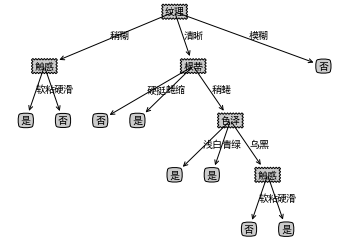
3. Results
dataSet, featureNames, featureNamesSet=readWatermelonDataSet()
testTree= createFullDecisionTree(dataSet, featureNames, featureNamesSet,featureNames)
createPlot(testTree)