In NLP tasks, the training data is usually one sentence (Chinese or English), and each step of input sequence data is one letter. We need to preprocess the data: first use the unique heat code for these letters, and then input it into RNN. For example, the letter a represents (1, 0, 0, 0,...) , 0), the letter b is (0, 1, 0, 0 , 0). If only the lowercase letters a~z are considered, the length of the input vector in each step is 26. If there are 1000 words in a sentence, we need to use the unique hot code of (1000,) dimension to represent each word.

Disadvantages:

• Every step of the input vector dimension will be very large
• In the unique heat representation, all words are equal, and the dependency between words is ignored

resolvent:

• Using word2vec, learn a mapping relationship F, and change a high-dimensional word (word) into a low-dimensional vector (vec=f(word).

Generally speaking, there are two ways to implement word embedding:

• Method based on "counting"
  • In a large corpus, the probability of one word and another word appearing at the same time is calculated, and the frequently occurring words are mapped to similar positions in vector space.
• Method based on "prediction"
  • Starting from one word or several words, we can predict their possible adjacent words, and naturally learn the mapping f of word embedding in the process of prediction.

The prediction based method is usually used. Specifically, there are two prediction based methods, CBOW and skip gram. Next, we will introduce their principles.

The principle of word embedding in CBOW

CBOW (Continuous Bag of Words) continuous bag model, which uses the context of a word to predict the word. For example: the manfill in love with the woman. If you only look at the first half of the sentence, that is, the man fill in love with the guy, you can probably guess that the line is "man". CBOW is to train a model to use context (in the above sentence, "the man fill in love with the") to predict possible words (such as woman).

First, consider using one word to predict the situation of another word. The corresponding network structure is shown in the figure below:

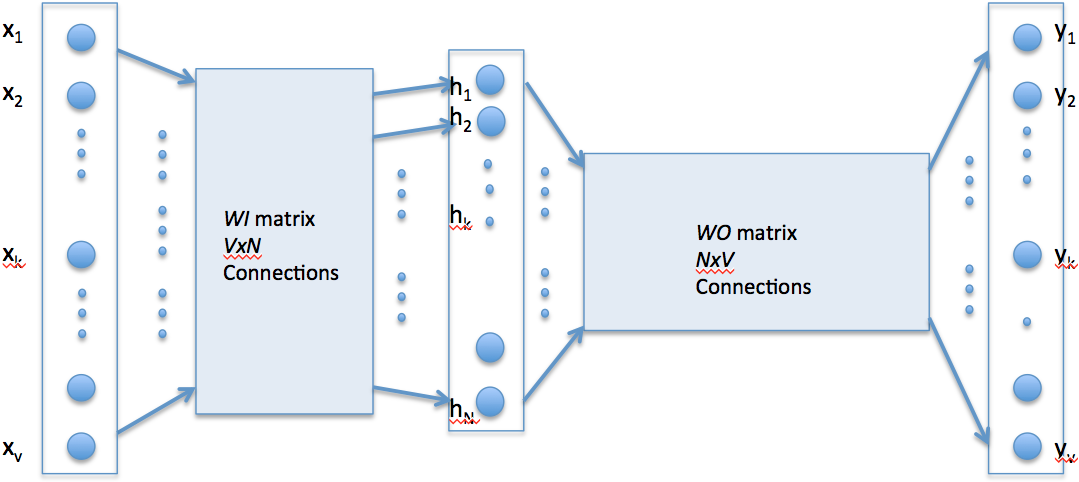
CBOW model: predicting a word with one word

In this case, the input word is still represented as x by the unique heat. Through a full connection layer, the hidden layer h is obtained, and then through a full connection layer, the output y is obtained.

V is the number of words in the vocabulary, so the dimension of x represented by Du hot is (V,). In addition, the output y is equivalent to the logits before Softmax operation, and its shape is also (V,), which uses one word to predict another word. The number of neurons in the hidden layer is n, and N is generally set to a value less than v. after training, the value of the hidden layer is regarded as an embedded representation of words, that is, "VEC" in word2vec.

How to use multiple words to predict a word? The answer is very simple. You can do the same full join operation on them first, and add up all the values to get the value of the hidden layer. The corresponding structure is shown in the figure below.

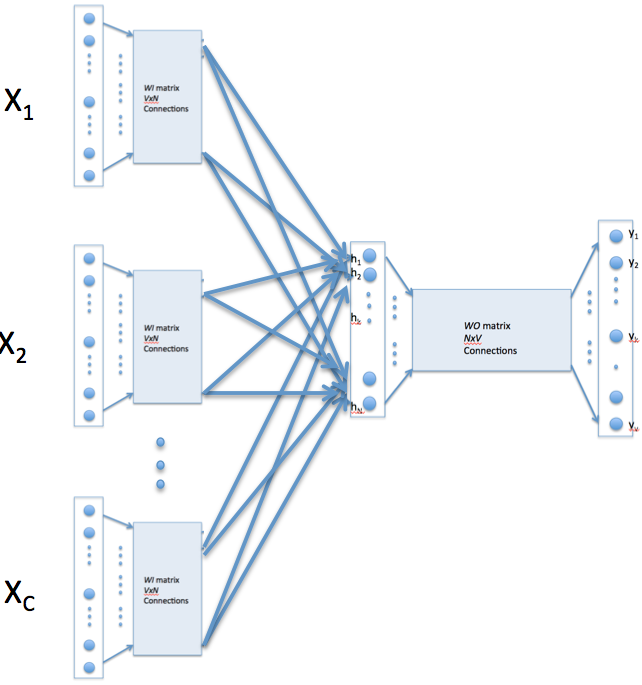
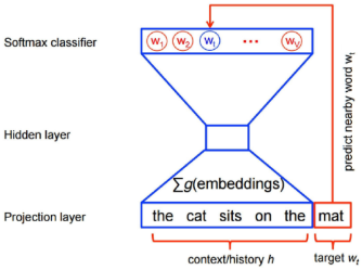
Left: CBOW model: use multiple words to predict a word; right: another representation of CBOW model

In the above figure, the context is "the cat bits on the", and the word to be predicted is "mat". σ g(embeddings) in the figure means adding up the embedded expressions of the, cat, bits, on and the five words (that is, adding the values of the hidden layer).

In the above structure, the whole network is equivalent to a V-Class classifier. V is the number of words in the word list. This value is often very large, so it is difficult to train. Usually, the structure of the network is simply modified, and the v-classification is changed into two categories.

Specifically, if the target word to be predicted is "mat", some words will be randomly selected as "noise words" in the whole word list, such as "computer", "boy" and "fork". There are two types of classification in the model: judging whether a word belongs to "noise word". Generally, if the context is h, the real target vocabulary corresponding to the context is $w_t $, the noise vocabulary is $\ tilde{w} $, and the optimization function is

$$J=\ln Q_{\theta}\left(D=1 | \boldsymbol{w}_{t}, \boldsymbol{h}\right)+k \underset{\tilde{\boldsymbol{w}}-P_{\min }}{E}\left[\ln Q_{\theta}(D=0 | \tilde{\boldsymbol{w}}, \boldsymbol{h})\right]$$

$Q {\ theta} \ left (D=1 | \ boldsymbol {w} {t}, \ boldsymbol {h} \ right) $represents the probability of a Logistic regression using the word embedding vector corresponding to the real word $W {T $and context $h $. Such Logistic regression can be regarded as a neural network. Because $w_t $is the real target word, you want the corresponding D=1. In addition, the noise word $\ tilde{w} $is not related to the sentence, so you want the corresponding D=0, that is $\ ln Q {\ theta} (D=0 | \ tilde{w} {t}, {h}) $. In addition, $\ understand {\ tilde{w} - P {noise}} {e} $indicates the expectation. It is impossible to accurately calculate such an expectation in the actual calculation. The usual way is to randomly take some noise words to estimate the expected value. The network structure corresponding to the loss is shown in the figure below.

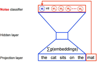
A CBOW model for two categories of noise words

After training the model by optimizing the biclassification loss function, the hidden layer in the final model can be regarded as "VEC" vector in word2vec. For a word, first input its unique representation into the model, and the value of the hidden layer is the corresponding word embedded representation. In addition, in TensorFlow, the loss used here is called NCE loss, and the corresponding function is tf.nn.nce_loss.

The principle of word embedding in skip gram

With the foundation of CBOW, the principle of skip gram is better understood. In CBOW method, context is used to predict the occurrence of words. For example, the context is "the man fill in love with the", and the word to be predicted is "woman". Skip gram method is the opposite of CBOW method: it uses "words that appear" to predict its "words in context". For example: the manfill in love with the woman. If you look only at the first half of the sentence, that is, the man fill in love with the \\\\\\\\\\. So, you can think of the skip gram method as a problem of predicting one word from another.

In terms of loss selection, like CBOW, we take out some "noise words" and train a two class classifier (that is, we also use NCE loss).

Word embedding in TensorFlow

Taking skip gram method as an example, we train a word embedding model in TensorFlow.

Download datasets

First, import some required libraries:

In order to train the language model with skip gram method, we need to download the corpus of the corresponding language. On the website http://mattmahoney.net/dc/ A large number of English corpora are available for download. To facilitate learning, a relatively small corpus is used http://mattmahoney.net/dc/text8.zip As an example training model. The program will automatically download this file:

# Step 1: Download the corpus at
url = 'http://mattmahoney.net/dc/'


def maybe_download(filename, expected_bytes):
    """
    //The functions of this function are:
        //If filename does not exist, download it at the address above.
        //If filename exists, skip the download.
        //Finally, it checks whether the bytes of the text are the same as expected_bytes.
    """
    if not os.path.exists(filename):
        print('start downloading...')
        filename, _ = urllib.request.urlretrieve(url + filename, filename)
    statinfo = os.stat(filename)
    if statinfo.st_size == expected_bytes:
        print('Found and verified', filename)
    else:
        print(statinfo.st_size)
        raise Exception(
            'Failed to verify ' + filename + '. Can you get to it with a browser?')
    return filename


# Download corpus text8.zip And verify the download
filename = maybe_download('text8.zip', 31344016)

Download corpus code

As stated in the comments, the program downloads the corpus from http://mattmahoney.net/dc/text8.zip and saves it as a text8.zip file. If text8.zip already exists in the current directory, it will not be downloaded. In addition, the program verifies that the number of bytes in text8.zip is correct.

If the reader finds that there is no way to download the file normally after running this program, he / she can try to download the file manually using the above url and place the downloaded file in the current directory.

After downloading and verification, use the following procedure to read out the data in the corpus:

#Decompress the corpus and convert it into a list of word s
def read_data(filename):
    """
    The functions of this function are:
        Extract the downloaded zip file and read it as a list of word s
    """
    with zipfile.ZipFile(filename) as f:
        data = tf.compat.as_str(f.read(f.namelist()[0])).split()
    return data


vocabulary = read_data(filename)
print('Data size', len(vocabulary)) (total length is about 17 million)
#Output the first 100 words.
print(vocabulary[0:100])

This program will unzip text8.zip and read it as a list in Python. Each element in the list is a word, such as:

This list of words is originally some consecutive sentences, but the punctuation is removed in the preprocessing of corpus. It is the original corpus.

Make a glossary

After downloading and taking out the corpus, we can make a word list. It can map the word to a number, which is the id of the word. If the original data is ['architect ',' original ',' as', 'a', 'term', 'of', 'abuse', 'first',...,], then the mapped data is [5234, 3081, 12, 6, 195, 2, 3134, 46,....], where 5234 represents the word architect, 3081 represents the word originated, and so on.

Generally speaking, because some words appear only a few times in the corpus, if the word list contains all the words in the corpus, it will be too large. Therefore, the word list generally contains only the most commonly used words. For the rest of the uncommon words, it will be replaced with a rare word mark "UNK". All rare words are mapped to the same word id.

The codes for making thesaurus and converting the previous corpus are as follows:

In this program, the word list contains only the 50000 most commonly used words. Note that in this implementation, the singular and plural forms of nouns (such as boy and boys) and the different tenses of verbs (such as make and make) are counted as different words. The original training data vocabulary is a list of words. After conversion, it becomes a list of word IDS, that is, the variable data in the program. Its form is [5234, 3081, 12, 6, 195, 23134, 46,...].

Generate training samples for each step

The variable data obtained in the previous step contains all the data in the training set. Now convert it to the batch data used in the training. A batch can be regarded as a set of "word pairs", such as woman - > man, woman - > fill. The left side of the arrow indicates "the word that appears", and the right side indicates the word in the context of the word. This is the skip gram method in section 14.2.2.

The detailed procedure of making training batch is as follows:

Although comments have been given in the code, in order to facilitate the reader's understanding, the code is further explained in detail. Here, a batch statement is generated as follows: batch, labels = generate ﹣ batch (batch﹣ size = 8, num ﹣ skips = 2, skip ﹣ window = 1). Each time the generate ﹣ batch function is run, a batch and corresponding labels will be generated. Note that the function has three parameters, batch_size, num_skips, and skip_window. The functions of these three parameters are described below.

The parameter batch Ou size should be understood best, which represents the number of word pairs in a batch. generate_batch returns two values, batch and labels. The former represents the "words appearing" in skip gram method, and the latter represents the words in context. Their shapes are (batch_size,) and (batch_size, 1), respectively.

Let's look at the parameters num? Skips and skip? Window. When generating word pairs, a list of continuous words with the length of skip_window*2+1 will be taken out in the corpus first, which is the variable buffer in the above program. The middle word in the buffer is "the word that appears" in the skip gram method, and the other two words of skip_window * are its "context". In the skip window * 2 words, randomly select num skips words and label them.

For example, in the case of skip window = 1 and num skips = 2. We will first select a buffer with a length of 3, assuming that it is ['analysis','originated ','as']. At this time, the original is the center word, and the remaining two words are its context. Then select num_skips from the two words to form a label. Because num_skips=2, only these two words can be selected in practice (the label cannot be repeated), and the final training data generated is originated - > analysis and originated - > as.

For another example, skip window = 3, Num skips = 2, we will first select a buffer with a length of 7, assuming that it is ['architect ',' originated ',' as', 'a', 'term', 'of', 'abuse']. At this time, the center word is a, and then randomly select two of the remaining words to form a word pair. For example, if you select term and of, the training data is a - > term, a - > of.

Because every time you select num_skips from skip*2 words, and the words cannot be repeated, you need skip_window * 2 > = num_skips. This is also reflected in the program (the corresponding statement is assert num? Skips < = 2 * skip? Window).

In the next training steps, the generate? Batch function is called once in each step, and the returned batch and labels are used as training data for training.

Define model

In fact, the model here can be abstracted as follows: one word is used to predict another word, and in the output, Softmax loss is not used, while NCE loss is used, that is, some "noise words" are selected as negative samples for two types of classification. The corresponding definition model code is:

First, we define an embedding variable whose shape is (vocabulary_size, embedding_size), which is equivalent to the embedding vector of a word in each line. For example, embedding with word id 0 is embeddings[0,:], embedding with word id 1 is embeddings[1,:], and so on. For the input data "train" inputs, a tf.nn.embedding "lookup function can be used to convert it into the corresponding word embedding vector embed according to the embeddings variable. By comparing the label of embedded and input data, we can directly define the NCE loss by tf.nn.NCE'loss function.

In addition, when training the model, we also want to verify the model. The method adopted here is to select some "verification words" and calculate the words closest to them in the embedding space. Because the directly obtained embeddings matrix may have different sizes in various dimensions, in order to make the calculated similarity more reasonable, we first normalize it, and then calculate the similarity between the verification words and other words with the normalized "embeddings".

Executive Training

After the model definition is completed, the training can be carried out, and the corresponding code is relatively simple:

Every 10000 steps, a verification will be performed, that is, select some "verification words", select the nearest words in the current embedding space, and output these words. For example, when the network is initialized (step=0), the validation output of the model is:

It can be found that these outputs are completely random and have no special significance.

But when the training reaches 100000 steps, the verification output becomes:

At this point, the vector representation in embedding space has some meaning. For example, which is closest to the word that, some is closest to many, and their is closest to its. These similarities are easy to understand. If the number of training steps is increased and the parameters in the model are adjusted reasonably, a more accurate word embedding representation will be obtained.

Finally, the resulting word embedding vector is final_embeddings, which is the normalized word embedding vector with the shape of (vocabulary_size,embedding_size), final_embeddings[0,:] is the word embedding representation corresponding to the word with id 0, final_embeddings[1,:] is the word embedding representation corresponding to the word with id 1, and so on.

visualization

In fact, the program can be finished after the final_embeddings are obtained, but it can go further to visualize the embedding space of words. Because of the embedding Gu size = 128 previously set, each word is represented as a 128 dimensional vector. Although there is no way to directly draw the 128 dimensional space, the following program uses the t-SNE method to map the 128 dimensional space to the 2-dimensional space, and draw the most commonly used 500 words. Save the picture as a tsne.png file:

When running this code, if it is executed by connecting to the server through ssh, errors like "RuntimeError: InvalidDISPLAY variable" may occur. At this time, you only need to add the following two statements before the statement "import matplotlib.pyplot as plt" to run successfully:

The generated "tsne.jpg" is shown in figure 14-5.

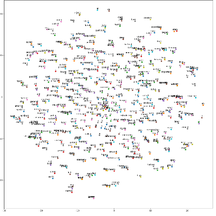
Using t-SNE method to visualize word embedding

The distance between similar words is relatively close. As shown in the figure below is the enlarged part of word embedding distribution.

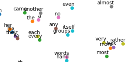
Embedded distribution of partial words after amplification

It is obvious that his, her, its and their words with similar parts of speech are put together.

In addition to similarity, there are some other interesting properties in the embedding space. As shown in figure 14-7, the corresponding relationships of man woman, King Queen, verb form, country and capital can be reflected in the embedding space.

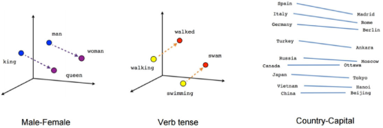
The correspondence in the embedding space of words

When training Char RNN in Chapter 12, we also mentioned "embedding" Chinese characters. What's the difference between embedding in Chapter 12 and word2vec in this chapter? In fact, whether in training CharRNN or in training word2vec model, a "word embedding layer" is added, but the objects are different - one is Chinese characters, the other is English words. The word embedding layer can embed Chinese or English words into a more dense space, which is helpful to improve the performance of the model. In Chapter 12, charrn's loss is used to train the model by predicting the characters at the next moment, and "bybelt" is embedded. In this chapter, the skip gram method is used to train word embedding by predicting the context of words.

Finally, if you want to train a CharRNN whose input unit is word (that is, the input of every step of the model is word, and the input of every step is word, not letter), then you can use the word embedding obtained in this chapter as the initial value of the word embedding layer of CharRNN to be trained, which can greatly improve the convergence speed. Similar methods can be adopted for Chinese characters or Chinese words.

I put the whole code here

# coding: utf-8

# Copyright 2015 The TensorFlow Authors. All Rights Reserved.
#
# Licensed under the Apache License, Version 2.0 (the "License");
# you may not use this file except in compliance with the License.
# You may obtain a copy of the License at
#
#     http://www.apache.org/licenses/LICENSE-2.0
#
# Unless required by applicable law or agreed to in writing, software
# distributed under the License is distributed on an "AS IS" BASIS,
# WITHOUT WARRANTIES OR CONDITIONS OF ANY KIND, either express or implied.
# See the License for the specific language governing permissions and
# limitations under the License.
# ==============================================================================
"""Basic word2vec example."""

# Import some required libraries
# from __future__ import absolute_import
# from __future__ import division
# from __future__ import print_function

import collections
import math
import os
import random
import zipfile

import numpy as np
from six.moves import urllib
from six.moves import xrange  # pylint: disable=redefined-builtin
import tensorflow as tf

# Step 1: Download the corpus at
url = 'http://mattmahoney.net/dc/'


def maybe_download(filename, expected_bytes):
    """
    //The functions of this function are:
        //If filename does not exist, download it at the address above.
        //If filename exists, skip the download.
        //Finally, it checks whether the bytes of the text are the same as expected_bytes.
    """
    if not os.path.exists(filename):
        print('start downloading...')
        filename, _ = urllib.request.urlretrieve(url + filename, filename)
    statinfo = os.stat(filename)
    if statinfo.st_size == expected_bytes:
        print('Found and verified', filename)
    else:
        print(statinfo.st_size)
        raise Exception(
            'Failed to verify ' + filename + '. Can you get to it with a browser?')
    return filename


# Download corpus text8.zip And verify the download
filename = maybe_download('text8.zip', 31344016)


# Decompress the corpus and convert it into a word Of list
def read_data(filename):
    """
    //The functions of this function are:
        //Extract the downloaded zip file and read it as a list of word s
    """
    with zipfile.ZipFile(filename) as f:
        data = tf.compat.as_str(f.read(f.namelist()[0])).split()
    return data


vocabulary = read_data(filename)
print('Data size', len(vocabulary))  # The total length is about 17 million
# Output the first 100 words.
print(vocabulary[0:100])

# Step 2: Make a list of words to turn the uncommon words into one UNK identifier 
# The size of the thesaurus is 50000 (i.e. we only consider the 50000 most frequently used words)
vocabulary_size = 50000


def build_dataset(words, n_words):
    """
    //Function function: change the original word representation into index
    """
    count = [['UNK', -1]]
    count.extend(collections.Counter(words).most_common(n_words - 1))
    dictionary = dict()
    for word, _ in count:
        dictionary[word] = len(dictionary)
    data = list()
    unk_count = 0
    for word in words:
        if word in dictionary:
            index = dictionary[word]
        else:
            index = 0  # UNK Of index For 0
            unk_count += 1
        data.append(index)
    count[0][1] = unk_count
    reversed_dictionary = dict(zip(dictionary.values(), dictionary.keys()))
    return data, count, dictionary, reversed_dictionary


data, count, dictionary, reverse_dictionary = build_dataset(vocabulary,
                                                            vocabulary_size)
del vocabulary  # Delete saved memory
# Output the 5 most common words
print('Most common words (+UNK)', count[:5])
# Output converted database data，And original words (top 10)
print('Sample data', data[:10], [reverse_dictionary[i] for i in data[:10]])
# Let's use data To make a training set
data_index = 0


# Step 3: define a function to generate skip-gram For model batch
def generate_batch(batch_size, num_skips, skip_window):
    # data_index Equivalent to a pointer, initially 0
    # Generate one at a time batch，data_index It's going to push back accordingly
    global data_index
    assert batch_size % num_skips == 0
    assert num_skips <= 2 * skip_window
    batch = np.ndarray(shape=(batch_size), dtype=np.int32)
    labels = np.ndarray(shape=(batch_size, 1), dtype=np.int32)
    span = 2 * skip_window + 1  # [ skip_window target skip_window ]
    buffer = collections.deque(maxlen=span)
    # data_index Is where the current data starts
    # produce batch Then push back 1 bit (generate batch)
    for _ in range(span):
        buffer.append(data[data_index])
        data_index = (data_index + 1) % len(data)
    for i in range(batch_size // num_skips):
        # utilize buffer generate batch
        # buffer Is a length of 2 * skip_window + 1 Of length word list
        # One buffer generate num_skips Number of samples
        #     print([reverse_dictionary[i] for i in buffer])
        target = skip_window  # target label at the center of the buffer
        #     targets_to_avoid Ensure that the sample is not repeated
        targets_to_avoid = [skip_window]
        for j in range(num_skips):
            while target in targets_to_avoid:
                target = random.randint(0, span - 1)
            targets_to_avoid.append(target)
            batch[i * num_skips + j] = buffer[skip_window]
            labels[i * num_skips + j, 0] = buffer[target]
        buffer.append(data[data_index])
        # Every use buffer generate num_skips Samples, data_index Just push back one bit
        data_index = (data_index + 1) % len(data)
    data_index = (data_index + len(data) - span) % len(data)
    return batch, labels


# By default skip_window=1, num_skips=2
# This is from the continuous 3(3 = skip_window*2 + 1)Generate 2 in words(num_skips)Samples.
# Like three consecutive words['used', 'against', 'early']
# Two samples are generated: against -> used, against -> early
batch, labels = generate_batch(batch_size=8, num_skips=2, skip_window=1)
for i in range(8):
    print(batch[i], reverse_dictionary[batch[i]],
          '->', labels[i, 0], reverse_dictionary[labels[i, 0]])

# Step 4: Model building.

batch_size = 128
embedding_size = 128  # Word embedding space is 128 dimensions. Namely word2vec Medium vec It's a 128 dimensional vector
skip_window = 1  # skip_window Parameters are the same as before
num_skips = 2  # num_skips Parameters are the same as before

# During training, the model will be verified 
# The way of verification is to find the word closest to a word.
# Front only valid_window Because these words are the most common
valid_size = 16  # 16 words at a time
valid_window = 100  # These 16 words are selected from the top 100 most common words
valid_examples = np.random.choice(valid_window, valid_size, replace=False)

# The number of noise words selected in loss construction
num_sampled = 64

graph = tf.Graph()

with graph.as_default():
    # Entered batch
    train_inputs = tf.placeholder(tf.int32, shape=[batch_size])
    train_labels = tf.placeholder(tf.int32, shape=[batch_size, 1])
    # Words for validation
    valid_dataset = tf.constant(valid_examples, dtype=tf.int32)

    # Some of the following functions have not gpu Implementation, so we only cpu Define model on
    with tf.device('/cpu:0'):
        # Define 1 embeddings Variable, which is equivalent to storing one word in one line embedding
        embeddings = tf.Variable(
            tf.random_uniform([vocabulary_size, embedding_size], -1.0, 1.0))
        # utilize embedding_lookup You can easily get one batch All words embedded in
        embed = tf.nn.embedding_lookup(embeddings, train_inputs)

        # Create two variables for NCE Loss(That is to say, the loss of dichotomies in selecting noise words)
        nce_weights = tf.Variable(
            tf.truncated_normal([vocabulary_size, embedding_size],
                                stddev=1.0 / math.sqrt(embedding_size)))
        nce_biases = tf.Variable(tf.zeros([vocabulary_size]))

    # tf.nn.nce_loss Noise words will be automatically selected and loss will be caused.
    # Random selection num_sampled Noise words
    loss = tf.reduce_mean(
        tf.nn.nce_loss(weights=nce_weights,
                       biases=nce_biases,
                       labels=train_labels,
                       inputs=embed,
                       num_sampled=num_sampled,
                       num_classes=vocabulary_size))

    # obtain loss After that, we can construct the optimizer
    optimizer = tf.train.GradientDescentOptimizer(1.0).minimize(loss)

    # Calculate word and word similarity (for validation)
    norm = tf.sqrt(tf.reduce_sum(tf.square(embeddings), 1, keep_dims=True))
    normalized_embeddings = embeddings / norm
    # Find and verify the embedding And calculate their similarity to all words
    valid_embeddings = tf.nn.embedding_lookup(
        normalized_embeddings, valid_dataset)
    similarity = tf.matmul(
        valid_embeddings, normalized_embeddings, transpose_b=True)

    # Variable initialization steps
    init = tf.global_variables_initializer()

# Step 5: start training
num_steps = 100001

with tf.Session(graph=graph) as session:
    # initialize variable
    init.run()
    print('Initialized')

    average_loss = 0
    for step in xrange(num_steps):
        batch_inputs, batch_labels = generate_batch(
            batch_size, num_skips, skip_window)
        feed_dict = {train_inputs: batch_inputs, train_labels: batch_labels}

        # Optimize one step
        _, loss_val = session.run([optimizer, loss], feed_dict=feed_dict)
        average_loss += loss_val

        if step % 2000 == 0:
            if step > 0:
                average_loss /= 2000
            # 2000 individual batch Average loss of
            print('Average loss at step ', step, ': ', average_loss)
            average_loss = 0

        # Every 10000 steps, we have a verification
        if step % 10000 == 0:
            # sim Is the similarity between the verification word and all words
            sim = similarity.eval()
            # There are valid_size Validation words
            for i in xrange(valid_size):
                valid_word = reverse_dictionary[valid_examples[i]]
                top_k = 8  # Output the most adjacent 8 words
                nearest = (-sim[i, :]).argsort()[1:top_k + 1]
                log_str = 'Nearest to %s:' % valid_word
                for k in xrange(top_k):
                    close_word = reverse_dictionary[nearest[k]]
                    log_str = '%s %s,' % (log_str, close_word)
                print(log_str)
    # final_embeddings It's the last thing we got embedding vector
    # Its shape is[vocabulary_size, embedding_size]
    # Each line represents the corresponding index Word embedding representation of words
    final_embeddings = normalized_embeddings.eval()


# Step 6: visualization
# The visual image will be saved as“ tsne.png"

def plot_with_labels(low_dim_embs, labels, filename='tsne.png'):
    assert low_dim_embs.shape[0] >= len(labels), 'More labels than embeddings'
    plt.figure(figsize=(18, 18))  # in inches
    for i, label in enumerate(labels):
        x, y = low_dim_embs[i, :]
        plt.scatter(x, y)
        plt.annotate(label,
                     xy=(x, y),
                     xytext=(5, 2),
                     textcoords='offset points',
                     ha='right',
                     va='bottom')

    plt.savefig(filename)


try:
    # pylint: disable=g-import-not-at-top
    from sklearn.manifold import TSNE
    import matplotlib
    matplotlib.use('agg')   # must be before importing matplotlib.pyplot or pylab
    import matplotlib.pyplot as plt

    # Because of our embedding Its size is 128 dimensions, so there is no way to directly visualize it
    # So we use t-SNE Method for dimensionality reduction
    tsne = TSNE(perplexity=30, n_components=2, init='pca', n_iter=5000)
    # Just 500 words
    plot_only = 500
    low_dim_embs = tsne.fit_transform(final_embeddings[:plot_only, :])
    labels = [reverse_dictionary[i] for i in xrange(plot_only)]
    plot_with_labels(low_dim_embs, labels)

except ImportError:
    print('Please install sklearn, matplotlib, and scipy to show embeddings.')

View Code

Reference resources

Thesis< Efficient Estimation of WordRepresentations in Vector Space >CBOW model and skip gram model