Word2vec of recommendation system
Objective: in the tasks related to natural language processing, we should hand over the natural language to the algorithm in machine learning. Usually, we need to mathematicize the language, because the machine is not a human, and the machine only recognizes mathematical symbols. Vectors are things that people abstract from nature and hand over to machines for processing. Basically, vectors are the main way of human input to machines.
Word vector is a way to mathematicize words in language. As the name suggests, word vector is to express a word as a vector. We all know that words need to be encoded into numerical variables before being sent to neural network training. There are two common coding methods: one hot representation and Distributed Representation
Disadvantages of OneHot coding:
- It is easily plagued by the disaster of dimensionality, especially when it is used in some algorithms of Deep Learning
When your vocabulary reaches tens of millions or even hundreds of millions, you will encounter a more serious problem, dimension explosion Here is an example of a word. You will find that we use four dimensions. When the number of words reaches tens of millions, the size of the word vector becomes tens of millions of dimensions. Without saying anything else, you can't stand such a large word vector in memory alone. If you use a bit to represent each dimension, a word needs about 0.12GB of memory, but note that this is only one word, there will be tens of millions of words in total, So the memory exploded. - The lexical gap can not well describe the similarity between words
Any two words are isolated. It is impossible to see whether the two words are related from these two vectors. For example, how can the relationship between I and like and the relationship between like and writing be expressed through 0001 and 0010 and 0010 and 0100, and through distance? Through the position of 1? You will find that single hot coding can't express any relationship between words at all. - Strong sparsity
When the dimension grows excessively, you will find that there are too many zeros. As a result, there is very little useful information in the whole vector, so it is almost impossible to calculate.
Due to the above problems of one hot coding, researchers will seek development in another way, namely Distributed Representation.
gensim package learning
import gensim
import seaborn as sns
import matplotlib.pyplot as plt
import jieba
import jieba.analyse
import logging
import os
from gensim.models import word2vec

from matplotlib import rcParams
config = {
    "font.family":'Times New Roman',  # Set font type
}
rcParams.update(config)
jieba.suggest_freq('Sarikin', True)
jieba.suggest_freq('Tian Guofu', True)
jieba.suggest_freq('Yu Liang Gao', True)
jieba.suggest_freq('Hou Liangping', True)
jieba.suggest_freq('Zhong Xiaoai', True)
jieba.suggest_freq('Yan Yan Chen', True)
jieba.suggest_freq('Ouyangjing', True)
jieba.suggest_freq('Easy to learn', True)
jieba.suggest_freq('Wang Dalu', True)
jieba.suggest_freq('Cai Chenggong', True)
jieba.suggest_freq('Sun Liancheng', True)
jieba.suggest_freq('Ji Changming', True)
jieba.suggest_freq('Ding Yizhen', True)
jieba.suggest_freq('Zheng Xipo', True)
jieba.suggest_freq('Zhao Donglai', True)
jieba.suggest_freq('Gao Xiaoqin', True)
jieba.suggest_freq('Zhao Ruilong', True)
jieba.suggest_freq('Hua Hua Lin', True)
jieba.suggest_freq('Lu Yiyi', True)
jieba.suggest_freq('Liu Xinjian', True)
jieba.suggest_freq('Liu celebration', True)

with open('./imgs/in_the_name_of_people.txt') as f:

    document = f.read()
    document_cut = jieba.cut(document)
    result = ' '.join(document_cut)
    with open('./imgs/in_the_name_of_people_segment.txt', 'w') as f2:
        f2.write(result)

f.close()
f2.close()
Building prefix dict from the default dictionary ...
Loading model from cache /tmp/jieba.cache
Loading model cost 0.838 seconds.
Prefix dict has been built successfully.
logging.basicConfig(format='%(asctime)s : %(levelname)s : %(message)s', level=logging.INFO)

sentences = word2vec.LineSentence('./imgs/in_the_name_of_people_segment.txt')

model = word2vec.Word2Vec(sentences
                          , sg=1
                          , min_count=1
                          , window=3
                          , size=100
                         )
# The most similar topk token s
model.wv.similar_by_word("Li Dakang", topn=5)
[('Qi Tongwei', 0.9853172302246094),
 ('Zhao Donglai', 0.9843684434890747),
 ('Ji Changming', 0.9813350439071655),
 ('Zheng Xipo', 0.9779636859893799),
 ('Tian Guofu', 0.9776411056518555)]
# Similarity between two word s
model.wv.similarity("Yu Liang Gao", "Wang Dalu")
0.9008845
plt.figure(figsize=(50, 2))
sns.heatmap(model.wv["Yu Liang Gao"].reshape(1, 100), cmap="Greens", cbar=True)

plt.figure(figsize=(50, 2))
sns.heatmap(model.wv["Wang Dalu"].reshape(1, 100), cmap="Greens", cbar=True)

# Not a group
model.wv.doesnt_match("Sha Ruijin, Gao Yuliang, Li Dakang, Liu Qingqing".strip().split())
'Liu celebration'
Word2Vec source code learning
Model: skip gram model based on Negative Sampling.
import collections
import math
import random
import sys
import time
import os
import numpy as np
import torch
from torch import nn
import torch.utils.data as Data
import matplotlib.pyplot as plt
import faiss


sys.path.append("..")
import d2lzh_pytorch as d2l
print(torch.__version__)
Processing data sets
assert 'ptb.train.txt' in os.listdir("../../data/ptb")
with open('../../data/ptb/ptb.train.txt', 'r') as f:
    lines = f.readlines()
    # st is the abbreviation of sentence
    # Read the words in each line
    raw_dataset = [st.split() for st in lines]

'# sentences: %d' % len(raw_dataset)
'# sentences: 42068'
for st in raw_dataset[:3]:
    print('# tokens:', len(st), st[:5])
# tokens: 24 ['aer', 'banknote', 'berlitz', 'calloway', 'centrust']
# tokens: 15 ['pierre', '<unk>', 'N', 'years', 'old']
# tokens: 11 ['mr.', '<unk>', 'is', 'chairman', 'of']
Build word index (low frequency processing)
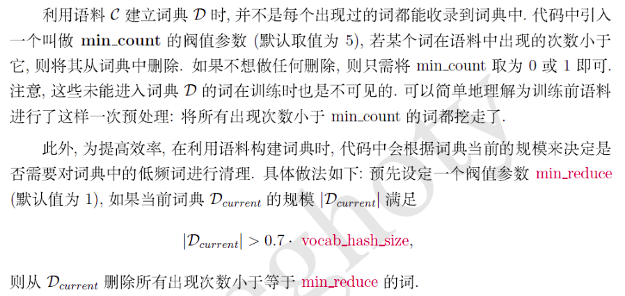
# tk is the abbreviation of token
# Build a word list, the number of words shall not be less than five (min_count), and the processing of low-frequency words
counter = collections.Counter([tk for st in raw_dataset for tk in st])
counter = dict(filter(lambda x: x[1] >= 5, counter.items()))
"""
counter data format
{'pierre': 6,
 '<unk>': 45020,
 'N': 32481,
 'years': 1241,
 'old': 268,
 """
# Establish the corresponding relationship between key and index value
idx_to_token = [tk for tk, _ in counter.items()]
token_to_idx = {tk: idx for idx, tk in enumerate(idx_to_token)}
len(idx_to_token)
9858
# The dataset is transformed into a dictionary with an id value
dataset = [[token_to_idx[tk] for tk in st if tk in token_to_idx]
           for st in raw_dataset]

# num_tokens indicates the total number of words
num_tokens = sum([len(st) for st in dataset])
'# tokens: %d' % num_tokens
'# tokens: 887100'
# Turn words into numeric indexes
dataset[1:3]
[[0, 1, 2, 3, 4, 5, 6, 7, 8, 9, 10, 11, 12, 13, 2],
 [14, 1, 15, 16, 17, 1, 18, 7, 19, 20, 21]]
Secondary sampling (processing of high-frequency words)
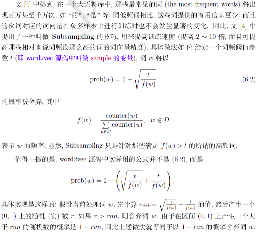
# Random value
random.uniform(0, 1)
0.13044269722038493
def discard(idx):
    """Discard some high-frequency words"""

    return random.uniform(0, 1) < 1 - math.sqrt(
        1e-4 / counter[idx_to_token[idx]] * num_tokens)

subsampled_dataset = [[tk for tk in st if not discard(tk)] for st in dataset]
'# tokens: %d' % sum([len(st) for st in subsampled_dataset])
'# tokens: 375873'
# Data content after sampling
subsampled_dataset[1:3]
[[0, 2, 4, 6, 8, 11], [16, 18, 7, 19, 20]]
#Comparison times
def compare_counts(token):

    return '# %s: before=%d, after=%d' % (token, sum(
        [st.count(token_to_idx[token]) for st in dataset]), sum(
        [st.count(token_to_idx[token]) for st in subsampled_dataset]))

compare_counts('the')
'# the: before=50770, after=2145'
compare_counts('join')
'# join: before=45, after=45'
Extract the head word and background word
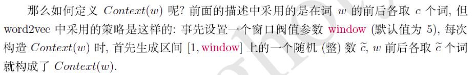
def get_centers_and_contexts(dataset, max_window_size):

    centers, contexts = [], []
    for st in dataset:
        if len(st) < 2:  # Each sentence must have at least two words to form a pair of "head word background word"
            continue
        centers += st
        for center_i in range(len(st)):
            window_size = random.randint(1, max_window_size)
            indices = list(range(max(0, center_i - window_size),
                                 min(len(st), center_i + 1 + window_size)))
            indices.remove(center_i)  # Exclude the head word from the background word
            contexts.append([st[idx] for idx in indices])

    return centers, contexts
tiny_dataset = [list(range(7)), list(range(7, 10))]
print('dataset', tiny_dataset)
for center, context in zip(*get_centers_and_contexts(tiny_dataset, 2)):
    print('center', center, 'has contexts', context)
dataset [[0, 1, 2, 3, 4, 5, 6], [7, 8, 9]]
center 0 has contexts [1]
center 1 has contexts [0, 2, 3]
center 2 has contexts [0, 1, 3, 4]
center 3 has contexts [2, 4]
center 4 has contexts [2, 3, 5, 6]
center 5 has contexts [4, 6]
center 6 has contexts [4, 5]
center 7 has contexts [8]
center 8 has contexts [7, 9]
center 9 has contexts [8]
all_centers, all_contexts = get_centers_and_contexts(subsampled_dataset, 5)
# [center] [context]
all_centers[1], all_contexts[1]
(2, [0, 4])
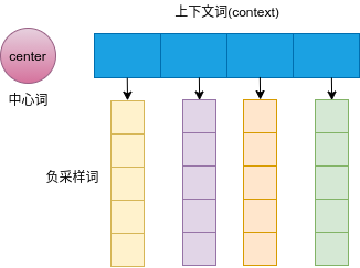
Negative sampling algorithm
Sampling idea:
First, the number of samples depends on the size of the data set. One experience is that for small data sets, 5-20 negative examples are selected, while for large data sets, only 2-5 negative examples are required. In addition, the sampling will follow a certain distribution. Here, the unigram distribution is used. Its characteristic is that words with higher word frequency are more likely to be selected as negative examples, which is a weighted sampling.
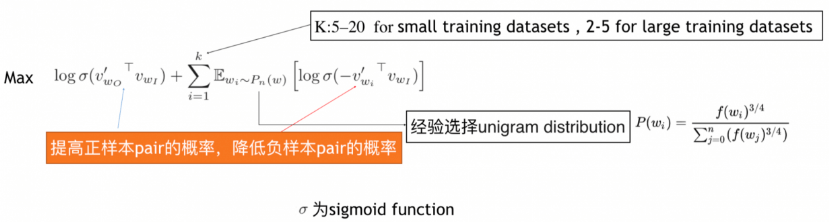
Negative sampling probability
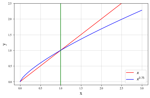
Design purpose of negative sampling frequency:
Add the 0.75 power of word frequency, slightly increase the sampling probability of low-frequency words, reduce the sampling probability of high-frequency words, down sample the high-frequency words, avoid the unnecessary calculation of these low information words, and avoid the excessive impact of high-frequency words on the model
P
(
w
i
)
=
c
o
u
n
t
e
r
(
w
i
)
3
4
∑
w
i
∈
D
c
o
u
n
t
e
r
(
w
i
)
3
4
P(w_i) = \frac{counter(w_i)^{\frac{3}{4}}}{\sum_{w_i\in{D}} counter(w_i)^{\frac{3}{4}}}
P(wi)=∑wi∈Dcounter(wi)43counter(wi)43
Sampling frequency diagram:
Negative sampling code
Objective: to sample several negative samples for each positive sample for parameter learning.
def get_negatives(all_contexts, sampling_weights, K):
    """
    all_contexts: Context words
    sampling_weights: Sampling weight
    K: Number of negative samples
    """

    all_negatives, neg_candidates, i = [], [], 0
    # Number of words
    population = list(range(len(sampling_weights)))
    for contexts in all_contexts:
        negatives = []
        #  Each positive sample samples K negative samples
        while len(negatives) < len(contexts) * K:
            if i == len(neg_candidates):
                # An index of k words is randomly generated as noise words according to the sampling_weights of each word.
                # For efficient calculation, k can be set slightly larger
                i, neg_candidates = 0, random.choices(
                    population, sampling_weights, k=int(1e5))

            neg, i = neg_candidates[i], i + 1
            # Noise words cannot be background words
            if neg not in set(contexts):
                negatives.append(neg)

        all_negatives.append(negatives)

    return all_negatives

# Count the word frequency (occurrence times) of each word, simplify the calculation, and the divisor is the same
sampling_weights = [counter[w]**0.75 for w in idx_to_token]  # molecule
all_negatives = get_negatives(all_contexts, sampling_weights, 5)
all_negatives[1]
[5, 4088, 3099, 6001, 341, 1094, 5015, 2, 3622, 53]
Binary cross entropy loss function
Loss function:
E
=
−
l
o
g
σ
(
v
o
′
T
h
)
−
∑
w
j
∈
W
n
e
g
l
o
g
σ
(
−
v
w
j
T
h
)
E = - log\sigma({v^{'}_o}^Th) - \sum_{w_j\in{W_{neg}}}log{\sigma(-v_{w_j}^Th})
E=−logσ(vo′Th)−wj∈Wneg∑logσ(−vwjTh)
class SigmoidBinaryCrossEntropyLoss(nn.Module):

    def __init__(self): # none mean sum

        super(SigmoidBinaryCrossEntropyLoss, self).__init__()

    def forward(self, inputs, targets, mask=None):
        """
        input – Tensor shape: (batch_size, len)
        target – Tensor of the same shape as input
        """

        inputs, targets, mask = inputs.float(), targets.float(), mask.float()
        res = nn.functional.binary_cross_entropy_with_logits(inputs, targets, reduction="none", weight=mask)

        return res.mean(dim=1)

loss = SigmoidBinaryCrossEntropyLoss()
pred = torch.tensor([[1.5, 0.3, -1, 2], [1.1, -0.6, 2.2, 0.4]])
# 1 and 0 in the label variable label represent background words and noise words respectively
label = torch.tensor([[1, 0, 0, 0], [1, 1, 0, 0]])
mask = torch.tensor([[1, 1, 1, 1], [1, 1, 1, 0]])  # Mask variable

loss(pred, label, mask) * mask.shape[1] / mask.float().sum(dim=1)
tensor([0.8740, 1.2100])
# Source form
def sigmd(x):

    return - math.log(1 / (1 + math.exp(-x)))

print('%.4f' % ((sigmd(1.5) + sigmd(-0.3) + sigmd(1) + sigmd(-2)) / 4)) # Note 1-sigmoid(x) = sigmoid(-x)
print('%.4f' % ((sigmd(1.1) + sigmd(-0.6) + sigmd(-2.2)) / 3))  # Divided by the number of valid values
0.8740
1.2100
Read data
def batchify(data):
    """be used as DataLoader Parameters of collate_fn: The input is a length of batchsize of list, list Every element in is__getitem__Results obtained"""

    max_len = max(len(c) + len(n) for _, c, n in data)
    centers, contexts_negatives, masks, labels = [], [], [], []

    for center, context, negative in data:
        cur_len = len(context) + len(negative)
        centers += [center]
        contexts_negatives += [context + negative + [0] * (max_len - cur_len)]
        # Mask mask to reduce unnecessary calculation
        masks += [[1] * cur_len + [0] * (max_len - cur_len)]
        labels += [[1] * len(context) + [0] * (max_len - len(context))]

    return (torch.tensor(centers).view(-1, 1), torch.tensor(contexts_negatives),
            torch.tensor(masks), torch.tensor(labels))
class MyDataset(torch.utils.data.Dataset):
    """custom dataset"""

    def __init__(self, centers, contexts, negatives):
        assert len(centers) == len(contexts) == len(negatives)
        self.centers = centers
        self.contexts = contexts
        self.negatives = negatives

    def __getitem__(self, index):
        return (self.centers[index], self.contexts[index], self.negatives[index])

    def __len__(self):
        return len(self.centers)

batch_size = 512
num_workers = 0 if sys.platform.startswith('win32') else 4

dataset = MyDataset(all_centers,
                    all_contexts,
                    all_negatives)

data_iter = Data.DataLoader(dataset, batch_size, shuffle=True,
                            collate_fn=batchify,
                            num_workers=num_workers)
for batch in data_iter:
    for name, data in zip(['centers', 'contexts_negatives', 'masks',
                           'labels'], batch):
        print(name, 'shape:', data.shape)
    break
centers shape: torch.Size([512, 1])
contexts_negatives shape: torch.Size([512, 60])
masks shape: torch.Size([512, 60])
labels shape: torch.Size([512, 60])
dataset[1]
(2, [0, 4], [5, 4088, 3099, 6001, 341, 1094, 5015, 2, 3622, 53])
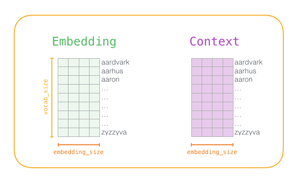
Skip word model
Embedded layer
# lookup table
embed = nn.Embedding(num_embeddings=20, embedding_dim=4)
embed.weight
Parameter containing:
tensor([[-0.9809,  0.0352, -0.4482,  1.9223],
        [ 0.4808,  1.1849,  1.8613,  0.9620],
        [ 1.8143, -0.6760,  0.3175, -0.7959],
        [-0.6967,  0.0555, -0.5704,  0.3390],
        [ 0.1333,  0.4522, -0.6569, -0.0352],
        [-0.8186, -0.7693, -0.2328, -0.2610],
        [-0.4525, -0.3535,  0.9490,  0.7209],
        [-2.3557,  0.0577,  0.8833, -0.5364],
        [-1.1420,  0.8997,  0.1042,  0.1357],
        [-0.4851,  0.6027,  0.1328, -0.1490],
        [ 0.4730, -1.6656, -2.3117,  1.4556],
        [ 1.4181, -0.0052, -1.3350,  0.1439],
        [ 0.9789, -0.8979,  2.9050, -2.4314],
        [-0.8238, -0.8194,  1.1061,  0.6439],
        [-0.4446,  0.1231,  0.2352, -0.6083],
        [ 1.0130,  0.4368,  0.3782, -0.8849],
        [-0.2142, -1.6758,  1.7204, -0.3238],
        [-0.9141, -0.5743,  0.1255,  0.3737],
        [-0.5698,  0.2665, -2.2218,  0.9601],
        [ 0.1554, -0.8226,  1.2788,  0.4957]], requires_grad=True)
x = torch.tensor([[1, 2, 3], [4, 5, 6]], dtype=torch.long)
em_x = embed(x)
em_x.shape
torch.Size([2, 3, 4])
Small batch multiplication
X = torch.ones((2, 1, 4))
Y = torch.ones((2, 4, 6))
torch.bmm(X, Y).shape
torch.Size([2, 1, 6])
Forward calculation of skip word model
Network architecture:
def skip_gram(center, contexts_and_negatives, embed_v, embed_u):

    v = embed_v(center)  # B * 1 * E
    u = embed_u(contexts_and_negatives) # B * C * E

    pred = torch.bmm(v, u.permute(0, 2, 1))  # B*1*C

    return pred
Training model
Initialize model parameters
embed_size = 100
net = nn.Sequential(
    nn.Embedding(num_embeddings=len(idx_to_token), embedding_dim=embed_size),
    nn.Embedding(num_embeddings=len(idx_to_token), embedding_dim=embed_size)
)
net
Sequential(
  (0): Embedding(9858, 100)
  (1): Embedding(9858, 100)
)
Define training function
def train(net, lr, num_epochs, plt = True):
    """
    train
    """

    device = torch.device('cuda' if torch.cuda.is_available() else 'cpu')
    print("train on", device)
    net = net.to(device)
    optimizer = torch.optim.Adam(net.parameters(), lr=lr)
    result_loss = []

    for epoch in range(num_epochs):
        start, l_sum, n = time.time(), 0.0, 0
        for batch in data_iter:
            # Each head word has several context words and noise words. The context is positive and the noise word is negative
            center, context_negative, mask, label = [d.to(device) for d in batch]
            pred = skip_gram(center, context_negative, net[0], net[1])
            # The mask variable mask is used to avoid the influence of padding on the calculation of loss function
            l = (loss(pred.view(label.shape), label, mask) *
                 mask.shape[1] / mask.float().sum(dim=1)).mean() # Average loss of a batch

            optimizer.zero_grad()
            l.backward()
            optimizer.step()
            l_sum += l.cpu().item()
            n += 1

        result_loss.append(l_sum / n)
        print('epoch %d, loss %.2f, time %.2fs'
              % (epoch + 1, l_sum / n, time.time() - start))

    return result_loss
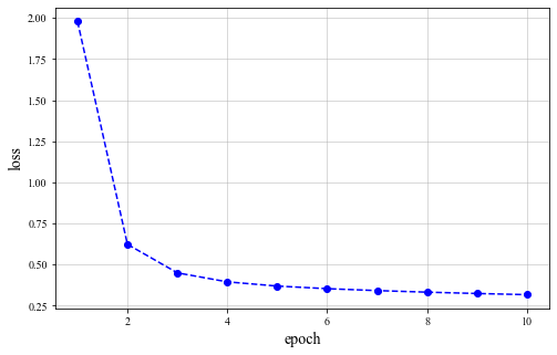
result_loss = train(net, 0.01, 10)
Loss change:
Applied word embedding model
cosine similarity
c o s ( θ ) = a ⋅ b ∣ ∣ a ∣ ∣ × ∣ ∣ b ∣ ∣ cos(\theta) = \frac{a\cdot{b}}{||a||\times||b||} cos(θ)=∣∣a∣∣×∣∣b∣∣a⋅b
def get_similar_tokens(query_token, k, embed):
    """Word embedding matrix"""

    W = embed.weight.data
    x = W[token_to_idx[query_token]]
    # 1e-9 is added for numerical stability (cosine similarity)

    cos = torch.matmul(W, x) / (torch.sum(W * W, dim=1) * torch.sum(x * x) + 1e-9).sqrt()
    _, topk = torch.topk(cos, k=k+1)
    topk = topk.cpu().numpy()

    for i in topk[1:]:  # Remove input words
        print('cosine sim=%.3f: %s' % (cos[i], (idx_to_token[i])))

get_similar_tokens('chip', 3, net[0])
cosine sim=0.537: intel
cosine sim=0.526: ibm
cosine sim=0.481: machines
Fiass lookup
Fiass - Faster search,Lower memory ,Run on GPUs
# Search by using fast embdeding similarity
def get_similar_tokens2faiss(token: str, topk = 5, embed = net[0]):

    lookup_table = embed.weight.data
    query_token = token
    x = lookup_table[token_to_idx[query_token]].view(1, -1).numpy()

    index = faiss.IndexFlatIP(embed_size)
    index.add(np.array(lookup_table))
    D, I = index.search(x=np.ascontiguousarray(x), k=topk)
    for i, (index, simi_value) in enumerate(zip(I[0], D[0])):
        if i == 0:
            continue
        print("sim dic: {}, value: {}".format(idx_to_token[index], simi_value))
get_similar_tokens2faiss(token = "chip", topk = 5, embed = net[0])
sim dic: flaws, value: 26.94745635986328
sim dic: intel, value: 22.954030990600586
sim dic: nugget, value: 22.86637306213379
sim dic: 30-share, value: 22.628337860107422
reference resources
Detailed explanation of mathematical principles in word2vec (key)
word2vec principle (I) basis of CBOW and skip gram model
Deep understanding of word2vec
Graphic Word2vec, reading this one is enough
heatmap
Summary of embedded technology practice of recommendation system
Application practice of EMBEDDING in Recommendation System
word2vec python implementation
Notes on formula derivation of Word2vec