- Word vector is a vector used to express the meaning of words, and can also be regarded as the feature vector of words. The technology of mapping words to real vectors is called word embedding.
1, Word embedding (Word2vec)
The unique heat vector can not accurately express the similarity between different words. word2vec is proposed to solve this problem. It maps each word to a fixed degree vector, which can better express the similarity and analogy between different words. word2vec contains two models: skip gram and CBOW. Their training depends on conditional probability. Because the data is not labeled, skip gram and CBOW are self-monitoring models.
1.Skip-Gram
Skip gram: the head word predicts the surrounding words
Every word has two
d
d
The vector representation of d dimension is used to calculate the conditional probability. For the index in the dictionary is
i
i
Any word of i, used separately
v
i
∈
R
d
\mathbf{v}_i\in\mathbb{R}^d
vi ∈ Rd and
u
i
∈
R
d
\mathbf{u}_i\in\mathbb{R}^d
ui ∈ Rd represents the two vectors when it is used as the head word and context word. Given central word
w
c
w_c
wc (subscript indicates the index in the dictionary) to generate any context word
w
o
w_o
The conditional probability of wo can be modeled by softmax operation on vector point product:
P
(
w
o
∣
w
c
)
=
exp
(
u
o
⊤
v
c
)
∑
i
∈
V
exp
(
u
i
⊤
v
c
)
(1)
P(w_o \mid w_c) = \frac{\text{exp}(\mathbf{u}_o^\top \mathbf{v}_c)}{ \sum_{i \in \mathcal{V}} \text{exp}(\mathbf{u}_i^\top \mathbf{v}_c)}\tag{1}
P(wo∣wc)=∑i∈Vexp(ui⊤vc)exp(uo⊤vc)(1)
Among them, thesaurus index set
V
=
{
0
,
1
,
...
,
∣
V
∣
−
1
}
\mathcal{V} = \{0, 1, \ldots, |\mathcal{V}|-1\}
V={0,1,...,∣V∣−1}.
Given length is
T
T
Text sequence of T, where time step
t
t
The word at t is
w
(
t
)
w^{(t)}
w(t). It is assumed that context words are generated independently given any central word. For context windows
m
m
m. The likelihood function of skip gram is the probability of generating all context words given any central word:
∏
t
=
1
T
∏
−
m
≤
j
≤
m
,
j
≠
0
P
(
w
(
t
+
j
)
∣
w
(
t
)
)
(2)
\prod_{t=1}^{T} \prod_{-m \leq j \leq m,\ j \neq 0} P(w^{(t+j)} \mid w^{(t)})\tag{2}
t=1∏T−m≤j≤m, j=0∏P(w(t+j)∣w(t))(2)
2.CBOW model
CBOW: prediction center word of surrounding words
Since there are multiple context words in CBOW, these context word vectors are averaged when calculating conditional probability. For index in dictionary i i Any word of i, respectively v i ∈ R d \mathbf{v}_i\in\mathbb{R}^d vi ∈ Rd and u i ∈ R d \mathbf{u}_i\in\mathbb{R}^d ui ∈ Rd represents two vectors used as context words and head words (the symbol is opposite to that in skip gram). Given context word w o 1 , ... , w o 2 m w_{o_1}, \ldots, w_{o_{2m}} wo1,..., wo2m (index in thesaurus is o 1 , ... , o 2 m o_1, \ldots, o_{2m} o1,..., o2m) generate any headword w c w_c The conditional probability of wc is:
P
(
w
c
∣
w
o
1
,
...
,
w
o
2
m
)
=
exp
(
1
2
m
u
c
⊤
(
v
o
1
+
...
,
+
v
o
2
m
)
)
∑
i
∈
V
exp
(
1
2
m
u
i
⊤
(
v
o
1
+
...
,
+
v
o
2
m
)
)
(3)
P(w_c \mid w_{o_1}, \ldots, w_{o_{2m}}) = \frac{\text{exp}\left(\frac{1}{2m}\mathbf{u}_c^\top (\mathbf{v}_{o_1} + \ldots, + \mathbf{v}_{o_{2m}}) \right)}{ \sum_{i \in \mathcal{V}} \text{exp}\left(\frac{1}{2m}\mathbf{u}_i^\top (\mathbf{v}_{o_1} + \ldots, + \mathbf{v}_{o_{2m}}) \right)}\tag{3}
P(wc∣wo1,...,wo2m)=∑i∈Vexp(2m1ui⊤(vo1+...,+vo2m))exp(2m1uc⊤(vo1+...,+vo2m))(3)
Given length is
T
T
Text sequence of T, where time step
t
t
The word at t is
w
(
t
)
w^{(t)}
w(t). For context windows
m
m
m. The likelihood function of CBOW is the probability of generating all central words given its context words:
∏ t = 1 T P ( w ( t ) ∣ w ( t − m ) , ... , w ( t − 1 ) , w ( t + 1 ) , ... , w ( t + m ) ) (4) \prod_{t=1}^{T} P(w^{(t)} \mid w^{(t-m)}, \ldots, w^{(t-1)}, w^{(t+1)}, \ldots, w^{(t+m)})\tag{4} t=1∏TP(w(t)∣w(t−m),...,w(t−1),w(t+1),...,w(t+m))(4)
2, Negative sampling and layered softmax
The main idea of skip gram is to use softmax operation to calculate the given central word w c w_c wc generate upper and lower text w o w_o Conditional probability of wo. Due to the nature of softmax operation, the context word can be a thesaurus V \mathcal{V} Any item in V contains the sum of as many items as the size of the whole thesaurus. Therefore, both skip gram gradient calculation and CBOW gradient calculation include summation. But usually a dictionary has hundreds of thousands or millions of words, and the computational cost of the gradient of summation is huge!
In order to reduce the computational complexity, take skip gram as an example to learn two approximate calculation methods: negative sampling and layered softmax.
1. Negative sampling
Given central word w c w_c wc's context window, any context word w o w_o wo. Events from this context window are considered to be modeled by the following probability:
P
(
D
=
1
∣
w
c
,
w
o
)
=
σ
(
u
o
⊤
v
c
)
=
exp
(
u
o
⊤
v
c
)
1
+
exp
(
u
o
⊤
v
c
)
=
1
1
+
exp
(
−
u
o
⊤
v
c
)
(5)
P(D=1\mid w_c, w_o) = \sigma(\mathbf{u}_o^\top \mathbf{v}_c)\\= \frac{\exp(\mathbf{u}_o^\top \mathbf{v}_c)}{1+\exp(\mathbf{u}_o^\top \mathbf{v}_c)}\\= \frac{1}{1+\exp(-\mathbf{u}_o^\top \mathbf{v}_c)}\tag{5}
P(D=1∣wc,wo)=σ(uo⊤vc)=1+exp(uo⊤vc)exp(uo⊤vc)=1+exp(−uo⊤vc)1(5)
Before negative sampling, softmax (multi classification) was used, and now sigmoid (two classification) is used.
Two categories and multiple categories can see the previous ones Logistic regression and multiple logistic regression This blog can be read in actual combat Logistic regression practice - stock customer churn early warning model (Python code) This.
Maximize the joint probability, and the given length is T T Text sequence of T w ( t ) w^{(t)} w(t) represents the time step t t The context window is m m m. The formula is:
∏
t
=
1
T
∏
−
m
≤
j
≤
m
,
j
≠
0
P
(
D
=
1
∣
w
(
t
)
,
w
(
t
+
j
)
)
(6)
\prod_{t=1}^{T} \prod_{-m \leq j \leq m,\ j \neq 0} P(D=1\mid w^{(t)}, w^{(t+j)})\tag{6}
t=1∏T−m≤j≤m, j=0∏P(D=1∣w(t),w(t+j))(6)
However, formula 6 considers only those events with positive samples. The joint probability is maximized to 1 only when all word vectors are equal to infinity. Of course, such a result is meaningless. To make the objective function more meaningful, negative sampling adds negative samples sampled from a predefined distribution.
use
S
S
S stands for context word
w
o
w_o
I'm from the head wo rd
w
c
w_c
The event of the context window of wc. For this involved
w
o
w_o
Events of wo , from predefined distribution
P
(
w
)
P(w)
Sampling in P(w)
K
K
K noise words not from this context window. use
N
k
N_k
Nk , stands for noise words
w
k
w_k
wk(
k
=
1
,
...
,
K
k=1, \ldots, K
k=1,..., K) is not from
w
c
w_c
The event of the context window of wc. Assume positive and negative cases
S
,
N
1
,
...
,
N
K
S, N_1, \ldots, N_K
S. These events of N1,..., NK... Are independent of each other. Negative sampling rewrites the joint probability (formula 2) of the original skip gram and changes the conditional probability to the following formula:
P
(
w
(
t
+
j
)
∣
w
(
t
)
)
≈
P
(
D
=
1
∣
w
(
t
)
,
w
(
t
+
j
)
)
∏
k
=
1
,
w
k
∼
P
(
w
)
K
P
(
D
=
0
∣
w
(
t
)
,
w
k
)
P(w^{(t+j)} \mid w^{(t)})\approx\\ P(D=1\mid w^{(t)}, w^{(t+j)})\prod_{k=1,\ w_k \sim P(w)}^K P(D=0\mid w^{(t)}, w_k)
P(w(t+j)∣w(t))≈P(D=1∣w(t),w(t+j))k=1, wk∼P(w)∏KP(D=0∣w(t),wk)
The loss function is negative log likelihood. Now the calculation cost of gradient is no longer related to the size of thesaurus, but to the number of noise words in negative sampling
K
K
K (is a super parameter,
K
K
The smaller the K, the lower the calculation cost).
2. Layered Softmax
Hierarchical Softmax uses a binary tree, where each leaf node of the tree represents a thesaurus
V
\mathcal{V}
A word in V.
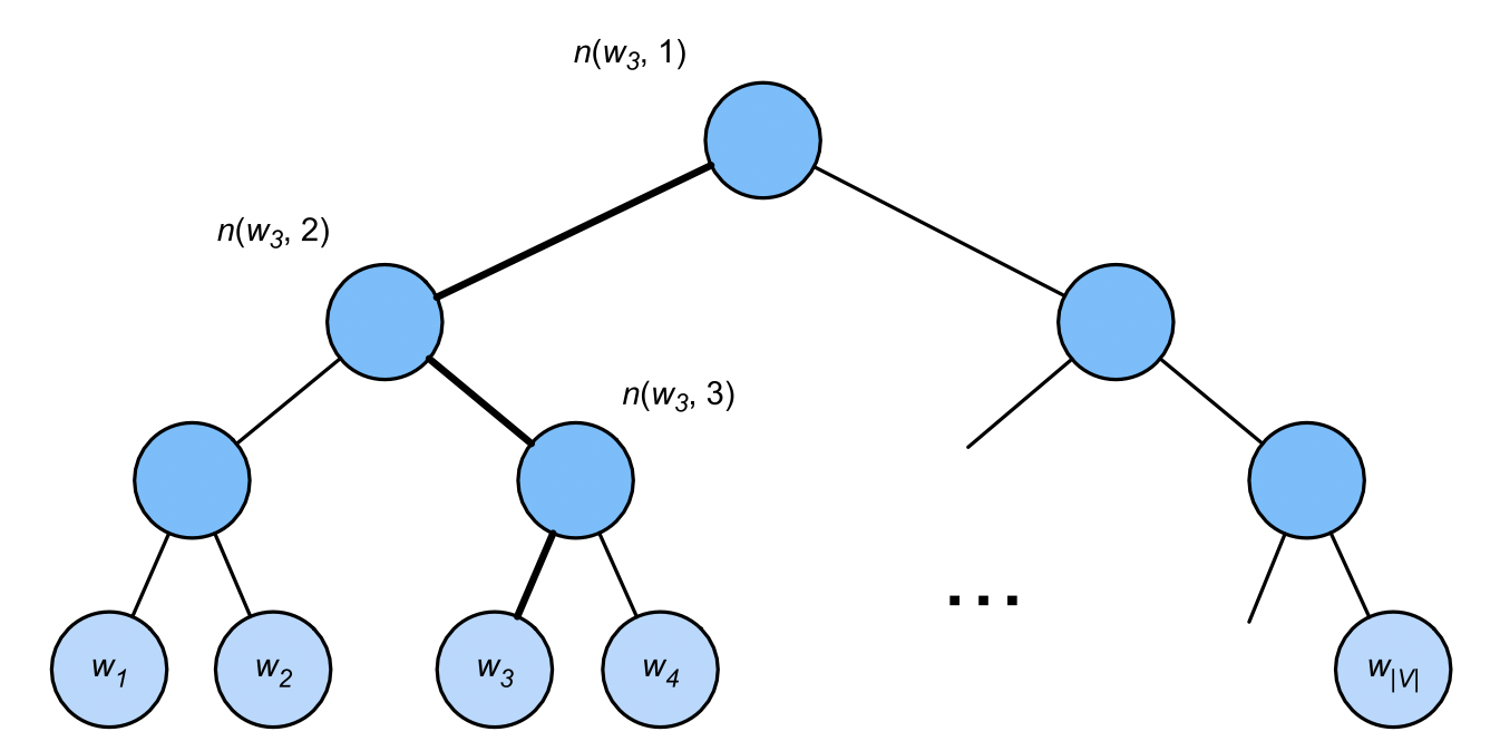
use L ( w ) L(w) L(w) represents a word in a binary tree w w w number of nodes on the path from root node to leaf node (including both ends). set up n ( w , j ) n(w,j) The path of (W) is n j t h j^\mathrm{th} jth node, whose upper and lower text vectors are u n ( w , j ) \mathbf{u}_{n(w, j)} un(w,j).
For example,
L
(
w
3
)
=
4
L(w_3) = 4
L(w3)=4. Layered softmax approximates the conditional probability as
P
(
w
o
∣
w
c
)
≈
∏
j
=
1
L
(
w
o
)
−
1
σ
(
[
[
n
(
w
o
,
j
+
1
)
=
leftChild
(
n
(
w
o
,
j
)
)
]
]
⋅
u
n
(
w
o
,
j
)
⊤
v
c
)
P(w_o \mid w_c) \approx \prod_{j=1}^{L(w_o)-1} \sigma\left( [\![ n(w_o, j+1) = \text{leftChild}(n(w_o, j)) ]\!] \cdot \mathbf{u}_{n(w_o, j)}^\top \mathbf{v}_c\right)
P(wo∣wc)≈j=1∏L(wo)−1σ([[n(wo,j+1)=leftChild(n(wo,j))]]⋅un(wo,j)⊤vc)
Among them,
leftChild
(
n
)
\text{leftChild}(n)
leftChild(n) is the node
n
n
Left child node of n: if
x
x
x is true,
[
[
x
]
]
=
1
[\![x]\!] = 1
[[x]]=1; otherwise
[
[
x
]
]
=
−
1
[\![x]\!] = -1
[[x]]=−1.
To calculate the given word in the figure above w c w_c wc generated word w 3 w_3 Take the conditional probability of w3 as an example. This requires w c w_c Word vector of wc + v c \mathbf{v}_c vc # and from root to w 3 w_3 The dot product between non leaf node vectors on the path of w3 (the path in bold in the figure), which traverses left, right and left in turn:
P
(
w
3
∣
w
c
)
=
σ
(
u
n
(
w
3
,
1
)
⊤
v
c
)
⋅
σ
(
−
u
n
(
w
3
,
2
)
⊤
v
c
)
⋅
σ
(
u
n
(
w
3
,
3
)
⊤
v
c
)
P(w_3 \mid w_c) = \sigma(\mathbf{u}_{n(w_3, 1)}^\top \mathbf{v}_c) \cdot \sigma(-\mathbf{u}_{n(w_3, 2)}^\top \mathbf{v}_c) \cdot \sigma(\mathbf{u}_{n(w_3, 3)}^\top \mathbf{v}_c)
P(w3∣wc)=σ(un(w3,1)⊤vc)⋅σ(−un(w3,2)⊤vc)⋅σ(un(w3,3)⊤vc)
from
σ
(
x
)
+
σ
(
−
x
)
=
1
\sigma(x)+\sigma(-x) = 1
σ (x)+ σ (− x)=1, which is based on arbitrary words
w
c
w_c
wc generate Thesaurus
V
\mathcal{V}
The sum of conditional probabilities of all words in V is 1:
∑
w
∈
V
P
(
w
∣
w
c
)
=
1.
\sum_{w \in \mathcal{V}} P(w \mid w_c) = 1.
∑w∈VP(w∣wc)=1.
In the binary tree structure, L ( w o ) − 1 L(w_o)-1 L(wo) − 1 is approximately the same as O ( log 2 ∣ V ∣ ) \mathcal{O}(\text{log}_2|\mathcal{V}|) O(log2 ∣ V ∣) is an order of magnitude. When thesaurus size V \mathcal{V} When V is large, the computational cost of each training step using layered softmax is significantly lower than that without approximate training.
Summary
- Negative sampling constructs the loss function by considering independent events, which involve both positive and negative cases. The calculation amount of training is linear with the number of noise words in each step.
- Hierarchical softmax uses the path from the root node to the leaf node in the binary tree to construct the loss function. The computational cost of training depends on the logarithm of the size of the thesaurus.
3, Data set for pre training word embedding
The dataset used here is Penn Tree Bank(PTB). The corpus is taken from the articles of the Wall Street Journal and is divided into training set, verification set and test set. In the original format, each line of the text file represents a sentence separated by spaces. Here, we treat each word as a word element.
import math
import os
import random
import torch
from torch import nn
from d2l import torch as d2l
from torch.nn import functional as F

d2l.DATA_HUB['ptb'] = (d2l.DATA_URL + 'ptb.zip',
                       '319d85e578af0cdc590547f26231e4e31cdf1e42')


def read_ptb():
    """take PTB The dataset is loaded into the list of text rows"""
    data_dir = d2l.download_extract('ptb')
    # Read the training set.
    with open(os.path.join(data_dir, 'ptb.train.txt')) as f:
        raw_text = f.read()
    return [line.split() for line in raw_text.split('\n')]
- Words constructed by "< unk > will appear less than 10 times.
sentences = read_ptb() # Number of sentances: 42069
vocab = d2l.Vocab(sentences, min_freq=10) # vocab size: 6719
1. Down sampling
Text data usually have high-frequency words such as "the", "a" and "in", which provide little useful information. In addition, a large number of (high frequency) words will make the training speed very slow. Therefore, when the training words are embedded in the model, the high-frequency words can be down sampled. That is, every word in the dataset w i w_i wi # will be discarded with probability
P
(
w
i
)
=
max
(
1
−
t
f
(
w
i
)
,
0
)
P(w_i) = \max\left(1 - \sqrt{\frac{t}{f(w_i)}}, 0\right)
P(wi)=max(1−f(wi)t
,0)
Among them,
P
(
w
i
)
P(w_i)
P(wi) is the probability of being discarded,
f
(
w
i
)
f(w_i)
f(wi) refers to the word
w
i
w_i
wi , frequency of occurrence in the dataset, constant
t
t
t is the super parameter (set to in the following code)
1
0
−
4
10^{-4}
10−4). Only when
f
(
w
i
)
>
t
f(w_i) > t
When f(wi) > t, (high frequency) words
w
i
w_i
wi can be discarded,
f
(
w
i
)
f(w_i)
The higher the f(wi), the higher the probability of being discarded.
- Down sampling high frequency words
def subsample(sentences, vocab):
    """Down sampling high frequency words"""
    # Exclude unknown word '< unk >'
    sentences = [[token for token in line if vocab[token] != vocab.unk]
                 for line in sentences]
    counter = d2l.count_corpus(sentences)
    num_tokens = sum(counter.values())

    # Returns True if word elements are retained during downsampling
    # Counter [token]: the frequency of tokens; num_tokens: total number of tokens (excluding < unk >)
    def keep(token):
        return(random.uniform(0, 1) <
               math.sqrt(1e-4 / counter[token] * num_tokens))

    return ([[token for token in line if keep(token)] for line in sentences],
            counter)

subsampled, counter = subsample(sentences, vocab)
- After down sampling, the number of samples of high-frequency words will be significantly reduced, while the number of samples of low-frequency words will not change and will be retained
def compare_counts(token):
    return (f'"{token}"Quantity of:'
            f'before={sum([l.count(token) for l in sentences])}, '
            f'after={sum([l.count(token) for l in subsampled])}')
'''
def compare_counts(token):
    return (f'"{token}"Quantity of:'
            f'before={counter[token]},'
            f'after={d2l.count_corpus(subsampled)[token]}')
'''
print(compare_counts('in'))
print(compare_counts('join'))
# Quantity of "in": before = 18000, after = 1191
# Quantity of "join": before = 45, after = 45
2. Extraction of head word and context word
The context window size is 1 to max_ window_ Random value of size
def get_centers_and_contexts(corpus, max_window_size):
    """return Skip-Gram Head word and context word"""
    centers, contexts = [], []
    for line in corpus:
        # To form a "head word context word" pair, each sentence needs to have at least 2 words
        if len(line) < 2:
            continue
        centers += line
        for i in range(len(line)):  # Context window middle i
            window_size = random.randint(1, max_window_size)
            indices = list(range(max(0, i - window_size),
                                 min(len(line), i + 1 + window_size)))
            # Exclude head words from context words
            indices.remove(i)
            contexts.append([line[idx] for idx in indices])
    # centers: contains all the words of corpus, and contexts: the context of all the central words
    return centers, contexts
3. Negative sampling
The noise words are sampled according to the predefined distribution, and the sampling distribution is through the variable sampling_weights transfer
class RandomGenerator:
    """according to n Sample weights in{1,...,n}Random sampling in"""
    def __init__(self, sampling_weights):
        # Exclude
        self.population = list(range(1, len(sampling_weights) + 1))
        self.sampling_weights = sampling_weights
        self.candidates = []
        self.i = 0

    def draw(self):
        if self.i == len(self.candidates):
            # Cache k random sampling results
            self.candidates = random.choices(
                self.population, self.sampling_weights, k=10000)
            self.i = 0
        self.i += 1
        return self.candidates[self.i - 1]
For a pair of head words and context words, random extraction K K K (5 in the experiment) noise words. According to the suggestions in the word2vec paper, the noise words w w Sampling probability of w P ( w ) P(w) P(w) is set to its relative frequency in the dictionary, and its power is 0.75.
def get_negatives(all_contexts, vocab, counter, K):
    """Returns the noise word in the negative sample"""
    # Index is 1, 2 (index 0 is an unknown tag excluded from the Thesaurus)
    sampling_weights = [counter[vocab.to_tokens(i)]**0.75
                        for i in range(1, len(vocab))]
    all_negatives, generator = [], RandomGenerator(sampling_weights)
    for contexts in all_contexts:
        negatives = []
        while len(negatives) < len(contexts) * K:
            neg = generator.draw()
            # Noise words cannot be context words
            if neg not in contexts:
                negatives.append(neg)
        all_negatives.append(negatives)
    return all_negatives
sentences = read_ptb()
vocab = d2l.Vocab(sentences, min_freq=10)
subsampled, counter = subsample(sentences, vocab)
# After down sampling, the lexical elements are mapped to their indexes in the corpus
corpus = [vocab[line] for line in subsampled]
all_centers, all_contexts = get_centers_and_contexts(corpus, 5)
all_negatives = get_negatives(all_contexts, vocab, counter, 5)
4. Small batch loading training examples
In small and medium batches, i t h i^\mathrm{th} The ith samples include the headwords and their n i n_i ni , contextual words and m i m_i mi # words noise. Due to the different size of the context window, n i + m i n_i+m_i ni + mi for different i i i is different. Therefore, for each sample, we are in contexts_negatives is a variable that links its context words and noise words and fills them with zero until the link length reaches max_len.
The mask variable masks is used to exclude padding when calculating losses. In order to distinguish positive and negative examples, labels variable is defined to separate context words from noise words. Where 1 in labels corresponds to contexts_ Positive examples of context words in negatives, and 0 corresponds to negative examples.
The input data is a list with a length equal to the batch size, in which each element is a sample composed of the central word center, its context word context and its noise word negative.
def batchify(data):
    """Returns a with a negative sample Skip-Gram Small batch samples"""
    max_len = max(len(c) + len(n) for _, c, n in data)
    centers, contexts_negatives, masks, labels = [], [], [], []
    for center, context, negative in data:
        cur_len = len(context) + len(negative)
        centers += [center]
        contexts_negatives += \
            [context + negative + [0] * (max_len - cur_len)]
        masks += [[1] * cur_len + [0] * (max_len - cur_len)]
        labels += [[1] * len(context) + [0] * (max_len - len(context))]
    return (torch.tensor(centers).reshape((-1, 1)), torch.tensor(
        contexts_negatives), torch.tensor(masks), torch.tensor(labels))
- The definition function reads the PTB data set and returns the data iterator and thesaurus
def load_data_ptb(batch_size, max_window_size, num_noise_words):
    """download PTB The dataset and then load it into memory"""
    sentences = read_ptb()
    vocab = d2l.Vocab(sentences, min_freq=10)
    subsampled, counter = subsample(sentences, vocab)
    corpus = [vocab[line] for line in subsampled]
    all_centers, all_contexts = get_centers_and_contexts(corpus, max_window_size)
    all_negatives = get_negatives(all_contexts, vocab, counter, num_noise_words)

    class PTBDataset(torch.utils.data.Dataset):
        def __init__(self, centers, contexts, negatives):
            assert len(centers) == len(contexts) == len(negatives)
            self.centers = centers
            self.contexts = contexts
            self.negatives = negatives

        def __getitem__(self, index):
            return (self.centers[index], self.contexts[index],
                    self.negatives[index])

        def __len__(self):
            return len(self.centers)

    dataset = PTBDataset(all_centers, all_contexts, all_negatives)
    data_iter = torch.utils.data.DataLoader(dataset, batch_size,
                                    shuffle=True, collate_fn=batchify)
    return data_iter, vocab
- Print the first small batch of data iterators
data_iter, vocab = load_data_ptb(512, 5, 5)
for batch in data_iter:
    for name, data in zip(names, batch):
        print(name, 'shape:', data.shape)
    break
centers shape: torch.Size([512, 1])
contexts_negatives shape: torch.Size([512, 60])
masks shape: torch.Size([512, 60])
labels shape: torch.Size([512, 60])
4, Pre training word2vec
batch_size, max_window_size, num_noise_words = 512, 5, 5
data_iter, vocab = d2l.load_data_ptb(batch_size, max_window_size, num_noise_words)
1. Forward communication
In the forward propagation, the input of skip gram includes the headword index center (batch size, 1) and the context and noise word index contexts_and_negatives (batch size, max_len). These two variables are first converted from the word element index into a vector through the embedding layer, and then their batch matrix is multiplied to return the output with the shape of (batch size, 1, max_len). Each element in the output is the dot product of the central word vector and the context or noise word vector.
def skip_gram(center, contexts_and_negatives, embed_v, embed_u):
    v = embed_v(center)
    u = embed_u(contexts_and_negatives)
    pred = torch.bmm(v, u.permute(0, 2, 1))
    return pred
2. Loss function
class SigmoidBCELoss(nn.Module):
    """Binary cross entropy loss with mask"""
    def __init__(self):
        super().__init__()

    def forward(self, inputs, target, mask=None):
        out = F.binary_cross_entropy_with_logits(
            inputs, target, weight=mask, reduction="none")
        return out.mean(dim=1)

loss = SigmoidBCELoss()
- Initialize model parameters
embed_size = 100
net = nn.Sequential(nn.Embedding(num_embeddings=len(vocab),
                                 embedding_dim=embed_size),
                    nn.Embedding(num_embeddings=len(vocab),
                                 embedding_dim=embed_size))
3. Training
def train(net, data_iter, lr, num_epochs, device=d2l.try_gpu()):
def init_weights(m):
if type(m) == nn.Embedding:
nn.init.xavier_uniform_(m.weight)
net.apply(init_weights)
net = net.to(device)
optimizer = torch.optim.Adam(net.parameters(), lr=lr)
animator = d2l.Animator(xlabel='epoch', ylabel='loss', xlim=[1, num_epochs])
# Sum of normalized losses
metric = d2l.Accumulator(2)
for epoch in range(num_epochs):
timer, num_batches = d2l.Timer(), len(data_iter)
for i, batch in enumerate(data_iter):
optimizer.zero_grad()
center, context_negative, mask, label = [data.to(device) for data in batch]
pred = skip_gram(center, context_negative, net[0], net[1])
l = (loss(pred.reshape(label.shape).float(), label.float(), mask)
/ mask.sum(axis=1) * mask.shape[1])
l.sum().backward()
optimizer.step()
metric.add(l.sum(), l.numel())
if (i + 1) % (num_batches // 5) == 0 or i == num_batches - 1:
animator.add(epoch + (i + 1) / num_batches,
(metric[0] / metric[1],))
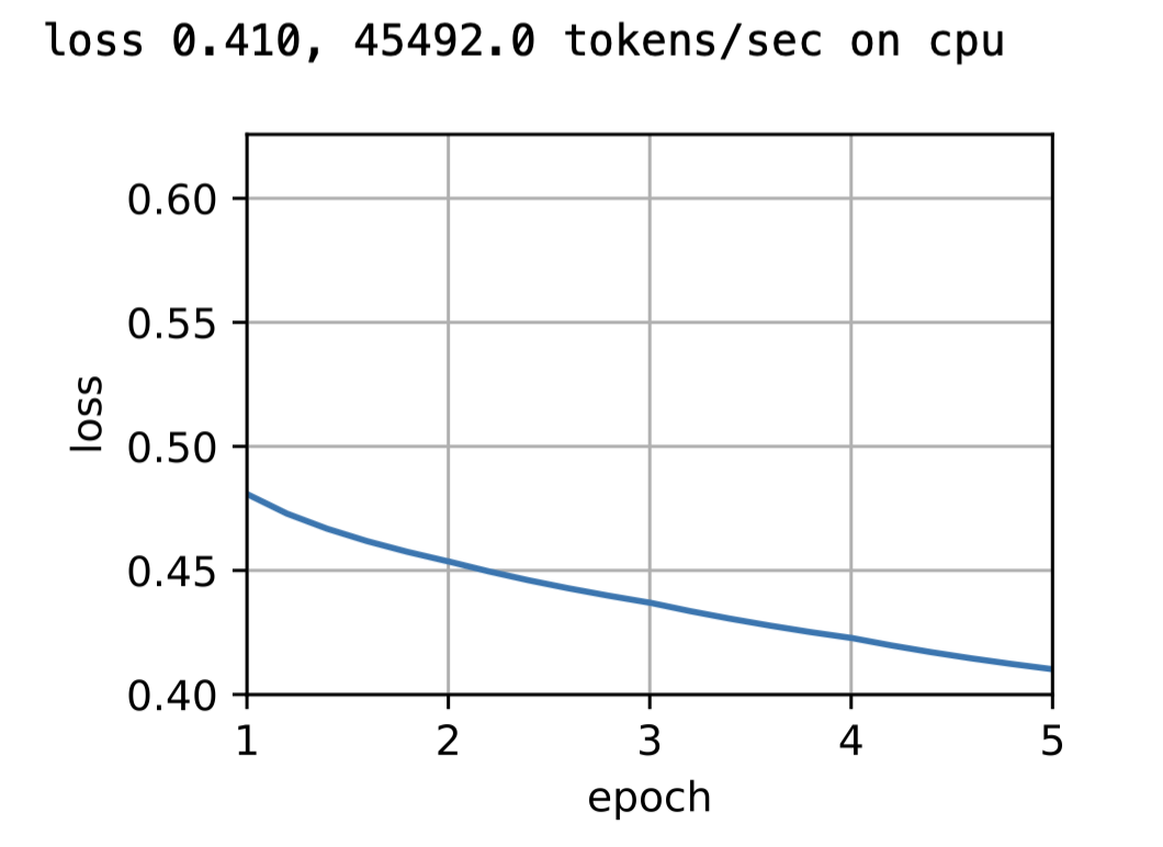
print(f'loss {metric[0] / metric[1]:.3f}, '
f'{metric[1] / timer.stop():.1f} tokens/sec on {str(device)}')
lr, num_epochs = 0.002, 5
train(net, data_iter, lr, num_epochs)
4. Application word embedding
After training the word2vec model, you can use the cosine similarity of the word vector in the trained model to find the word with the most similar semantics to the input word from the thesaurus.
def get_similar_tokens(query_token, k, embed):
    W = embed.weight.data
    x = W[vocab[query_token]]
    # Calculate cosine similarity. Add 1e-9 for numerical stability
    cos = torch.mv(W, x) / torch.sqrt(torch.sum(W * W, dim=1) *
                                      torch.sum(x * x) + 1e-9)
    # torch.topk(cos, k=k+1)[1] returns the first k+1 corresponding indexes in descending order
    topk = torch.topk(cos, k=k+1)[1].cpu().numpy().astype('int32')
    for i in topk[1:]:  # Delete input word
        print(f'cosine sim={float(cos[i]):.3f}: {vocab.to_tokens(i)}')

get_similar_tokens('chip', 3, net[0])